Evaluation
Introduction
Use the insurance scheme designed in the previous chapter.
First load the mortality predictions data.
d <- readRDS("pred_mort1.rds")
d <- na.omit(d)
Compute mortality losses as the difference between the observed mortality (mortality_rate) and the trigger we adopted previously. Subsequently, compute insurance pay as estimated from predicted mortality (predicted_mortality) using the same trigger.
trigger <- 0.20
d$loss <- pmax(0, d$mortality_rate - trigger)
d$pay  <- pmax(0, d$predicted_mortality - trigger)
head(d, n=2)
##   year season sublocation      NDVI year_season stock_beginning       loss
## 1 2008   SRSD      BUBISA 1.4511091   2008_SRSD           168.3 0.00000000
## 2 2008   SRSD DIRIB GOMBO 0.9011262   2008_SRSD           118.3 0.07303467
##   mortality_rate predicted_mortality         pay
## 1     0.09150327           0.1797705 0.000000000
## 2     0.27303467           0.2016966 0.001696612
Below is a plot of pay as computed from predicted mortality versus observed. Ideally, if predictions are the same as observed then their plot should form a straight line.
plot(d$loss, d$pay, xlab="Loss", ylab="Pay")
abline(0,1, col="red")
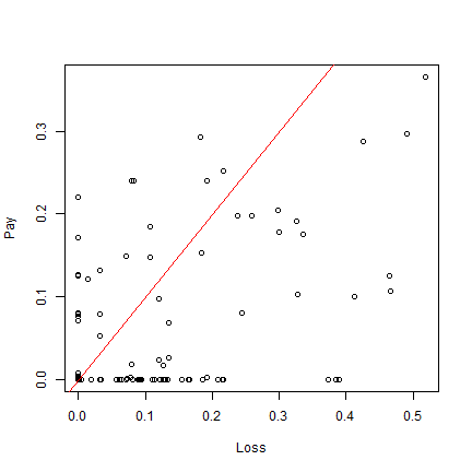
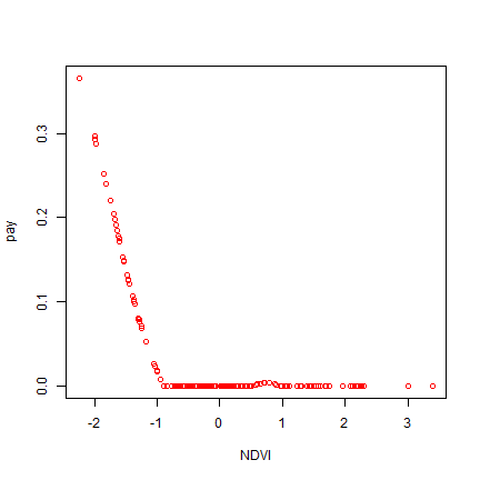
What do you make of the plots? What of a plot of payouts versus zNDVI?
plot(pay~NDVI, data=d, col="red")
We now need to assess the welfare of index insurance to the pastoralists. We use the certainty equivalent function.
library(agro)
agro::ce_income
## function (income, rho)
## {
##     u <- utility(income, rho, scale = FALSE)
##     ce_utility(u, rho)
## }
## <bytecode: 0x000001e99a16eaa8>
## <environment: namespace:agro>
Let us compute the premium that is paid for IBLI insurance as equivalent to the expected payouts with a mark up of 25%. We will basically compare the IBLI welfare based on the observed mortality (base) and predicted mortality (insurance).
markup <- 0.25
premium <- mean(d$pay) * (1 + markup)
premium
## [1] 0.04596454
base <- 1-d$mortality_rate
insurance_nomarkup <- base + d$pay
insurance <- insurance_nomarkup - premium
base <- base * 100
insurance <- insurance * 100
insurance_nomarkup <- insurance_nomarkup * 100
Compute CE with insurance (insurance) and without (base) respectively and compare them based on \(\rho\).
rho <- 2
ce_base <- ce_income(base, rho)
ce_ins25  <- ce_income(insurance, rho)
ce_ins_nomarkup  <- ce_income(na.omit(insurance_nomarkup), rho)
ce_base
## [1] 73.25194
ce_ins25
## [1] 74.03087
ce_ins_nomarkup
## [1] 78.85488
ce_ins25 / ce_base
## [1] 1.010634
ce_ins_nomarkup/ce_base
## [1] 1.076489
head(d, n=2)
##   year season sublocation      NDVI year_season stock_beginning       loss
## 1 2008   SRSD      BUBISA 1.4511091   2008_SRSD           168.3 0.00000000
## 2 2008   SRSD DIRIB GOMBO 0.9011262   2008_SRSD           118.3 0.07303467
##   mortality_rate predicted_mortality         pay
## 1     0.09150327           0.1797705 0.000000000
## 2     0.27303467           0.2016966 0.001696612
Compute CE over \(0 \leq \rho \leq 10\) and plot CE pay percentage when there is no mark up on insurance (ce_ins_nomarkup), when insurance is 25% marked up (ce_ins) and a case where no insurance is taken by pastrolist (ce_base).
rhos <- seq(0, 3, .1)
ce_base <- ce_ins <- ce_ins_nomarkup <- rep(NA, length(rhos))
for(i in 1:length(rhos)){
  ce_base[i] <- ce_income(base, rhos[i])
  ce_ins[i]  <- ce_income(insurance, rhos[i])
  ce_ins_nomarkup[i] <- ce_income(insurance_nomarkup, rhos[i])
}
inc <- seq(0.1, 1, 0.1)
plot(rhos, ce_base, type="l", col="blue", ylab= "Pay (%)", xlab="CRRA", cex=2, ylim=c(70, 90))
lines(rhos, ce_ins, col="red")
lines(rhos, ce_ins_nomarkup, col="green")
legend("topright", c("No insurance", "25% Marked-up Insurance", "No mark up"), lty=1, col=c("blue", "red", "green"), title = "IBLI contract type", bty = "n")
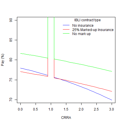
What do you observe from the graphs? What happens when you change the trigger to say 20%?
Let do the MQS test using the same values of CRRA and make a plot to determine pastrolist welfare with and without insurance.
ce_base <- ce_ins <- mqs <- rep(NA, length(rhos))
for(i in 1:length(rhos)){
  ce_base[i] <- ce_income(base, rhos[i])
  ce_ins[i]  <- ce_income(insurance, rhos[i])
  mqs[i] <- ce_ins[i] - ce_base[i]
}
inc <- seq(0.1, 1, 0.1)
plot(rhos, mqs*100, type="l", col="blue", ylab= "MQS (insurance benefit in %)", xlab="CRRA", cex=2)
abline(h=0, col="red")
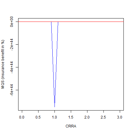
From the plot you can observe that pastoralists with a risk aversion less than 1.5 do not derive any value from the insurance. However, those with higher risk aversion derive more benefit from the insurance as the fall above the zero line.
Simulation
Remember we predicted mortality previously based on zNDVI however there is uncertainty that is associated with our model. We will therefore conduct a simulation of pay based on 95% confidence interval of the model’s predictions.
Let us set up the environment including required library and data.
library(msir)
## Warning: package 'msir' was built under R version 4.3.1
dd <- na.omit(d)
Create a model that predicts mortality from zNDVI.
m <- loess.sd(dd$NDVI, dd$mortality_rate)
fitsd <- cbind(fit=m$model$fitted, sd=m$sd)
Let us sample 1000 times from the model we created previously.
ns <- 1000
sample <- apply(fitsd, 1, function(i) {
  pmin(1, pmax(0, rnorm(ns, i[1], i[2])))
})
sample <- t(sample)
Compute insurance premium with 25% and with no markup from the samples
markup <- 0.2
premium <- mean(dd$pay) * (1 + markup)
and their corresponding CE at \(\rho=2\).
out_nomarkup <- out_ins <- out_base <- rep(NA, ns)
rho = 2
for (i in 1:ns) {
  base <- 1- sample[,i]
  insurance_nomarkup <- base + dd$pay
  insurance <- insurance_nomarkup - premium
  out_base[i] <- ce_income(100*base, rho)
  out_ins[i]  <- ce_income(100*insurance, rho)
  out_nomarkup[i]  <- ce_income(100*insurance_nomarkup, rho)
}
mean(out_base)
## [1] 73.34839
mean(out_ins)
## [1] 74.3992
mean(out_nomarkup)
## [1] 78.96075
Make some plots.
benefit_ins <- out_ins - out_base
benefit_nomu <- out_nomarkup - out_base
b <- cbind(benefit_ins, benefit_nomu)
boxplot(b, ylim=c(-1,10))
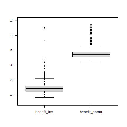
The graph illustrates that the contract passes the welfare MQS test.