Spatio-temporal aggregation
Temporal NDVI aggregate
For the entire analysis we use precomputed NDVI for the period between 2008 to 2015. The next code block downloads the pre-processed data. The first time this takes a while. After that, it should be quick as the data won’t be downloaded again if they are still on your disk.
library(terra)
datadir <- "modis"
files <- agrodata::data_ibli("marsabit_modis_ndvi", datadir)
head(basename(files))
## [1] "MOD09A1.A2008065.h21v08.006.2015172190147_ndvi.tif"
## [2] "MOD09A1.A2008073.h21v08.006.2015172214511_ndvi.tif"
## [3] "MOD09A1.A2008081.h21v08.006.2015172215738_ndvi.tif"
## [4] "MOD09A1.A2008089.h21v08.006.2015173033705_ndvi.tif"
## [5] "MOD09A1.A2008097.h21v08.006.2015173034204_ndvi.tif"
## [6] "MOD09A1.A2008105.h21v08.006.2015173092905_ndvi.tif"
Get the area of interest again. We project to the sinusoidial coordinate refrence system that the MODIS data are in
aoi <- agrodata::data_ibli("marsabit")
sinprj <- "+proj=sinu +lon_0=0 +x_0=0 +y_0=0 +a=6371007.181 +b=6371007.181 +units=m +no_defs "
pols <- project(aoi, sinprj)
Now set up some parameters to select the subsets of files that we need.
# Define time period
startyear <- 2008
endyear   <- 2015
# Define a season (LRLD in this case)
sSeason <- "LRLD"
startSeason <- "03-01"
endSeason   <- "09-30"
Below we define a function for selecting MODIS files for a given year and season.
library(luna)
library(meteor)
selectModisFiles <- function(files, startdate, enddate) {
  base_names <- basename(files)
  dates <- luna::dateFromYearDoy(substr(base_names, 10, 16))
  i <- (dates >= as.Date(startdate)) & (dates <= as.Date(enddate) )
  files[i]
}
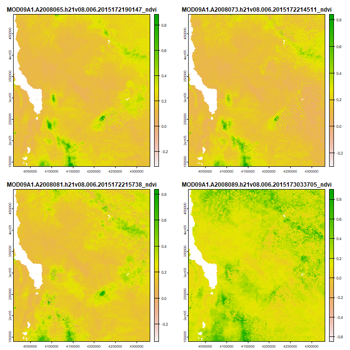
Let’s try the function. First for a single year, and to make a plot
season <- selectModisFiles(files, paste0(startyear, "-", startSeason), paste0(startyear, "-", endSeason))
sndvi <- rast(season)
plot(sndvi[[1:4]])
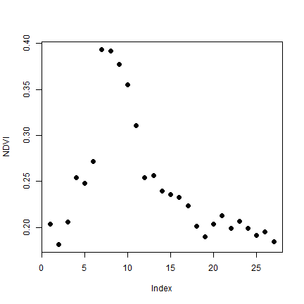
We can compute 8-day NDVI spatial aggregates by region.
ndvi_val <- terra::extract(sndvi, pols, fun=mean, na.rm=TRUE)
# the first region
plot(unlist(ndvi_val[1, -1]), ylab= "NDVI", pch=20, cex=2)
Now, we process all files
workdir <- "work"
dir.create(workdir, recursive=TRUE, showWarnings=FALSE)
for(year in startyear:endyear) {
  season <- selectModisFiles(files, paste0(year, "-", startSeason), paste0(year, "-", endSeason))
  sndvi <- rast(season)
  ndvimean <- mean(sndvi, na.rm = TRUE)
  # Shorten layer names
  names(sndvi) <- paste0("ndvi_", luna::dateFromYearDoy(substr(names(sndvi), 10, 16)))
  filename=file.path(workdir, paste0( 'MOD09A1.h21v08.',year,"_",sSeason,'_ndvit.tif'))
  writeRaster(ndvimean, filename = filename , overwrite=TRUE)
}
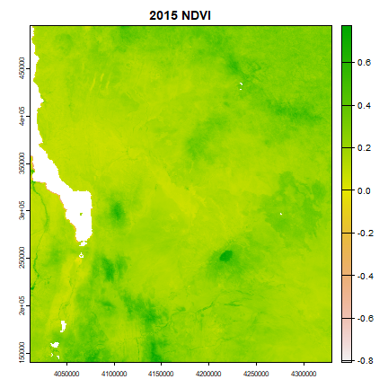
Here is an example of the files we have created.
par(mar = c(2.2, 2.2, 1.2, 0.5)) #c(bottom, left, top, right)
stitle <- paste(year, " NDVI", sep="")
plot(ndvimean, main = stitle)
Spatial aggregation
Above we computed the seasonal mean NDVI for each pixel. Next we compute spatially aggregated NDVI for each sub-location.
season <- "LRLD"
files <- list.files(workdir, pattern=paste0(season,"_ndvit.tif$"), full.names=TRUE)
ndvi <- rast(files)
# Compute spatial aggregates by sub-location
output <- extract(ndvi, pols, fun=mean, na.rm=TRUE)
# remove the first column with IDs
output <- output[,-1]
colnames(output) <- substr(basename(files),16,19)
output[1:3, 1:6]
##        2008      2009      2010      2011      2012      2013
## 1 0.2452315 0.1858393 0.2626484 0.1909502 0.2426913 0.2557569
## 2 0.3145086 0.2174733 0.3068873 0.1835347 0.4313131 0.4081481
## 3 0.1704560 0.1377076 0.2692909 0.1392298 0.1546021 0.1832170
Now we combine the aggregated data with the polygon data, and we save it to disk as we might want to use it again later.
# Create a data.frame
res <- data.frame(SLNAME=pols$SUB_LOCATION, IBLI_Zone=pols$IBLI_UNIT, output, stringsAsFactors = FALSE, check.names=FALSE)
saveRDS(res, file.path(workdir, paste0(season,"_ndvi_st_mat.rds")))
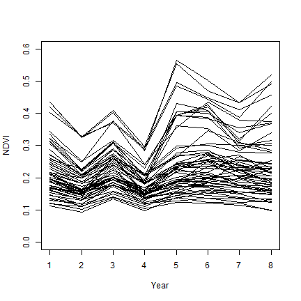
Now we can plot the seasonal mean NDVI over time, by region.
output <- as.matrix(output)
plot(output[1,], ylab="NDVI", xlab="Year", type="l", ylim=c(0,.6))
for (i in 2:nrow(output)) {
  lines(output[i,])
}
Z-scores
Now we can compute z-scores based on the period 2008–2015 as an example. Z-scores indicate the deviations of seasonal NDVI from its longterm annual mean. The unit is “standard deviations”. This a z-score of -1 means that the value is 1 standard deviation below the (expected) mean value.
z-score computation function:
zscore <- function(y){
  (y - mean(y, na.rm=TRUE) ) / (sd(y, na.rm=TRUE))
}
Now we can use this function to compute z-scores over the LRLD period. You can also make some plots to assess forage availablity. For instance, assume a threshold of zero and make payouts anytime the zonal mean deviates below the historical average. In addition, instead of simple line plot you can use linear regression and some local smoothing functions like moving average.
scores <- apply(res[,-c(1:2)], 1, zscore)
scores <- t(scores)
scores[1:5, 1:6]
##             2008       2009       2010       2011       2012      2013
## [1,]  0.51837896 -1.5372188  1.1211886 -1.3603279  0.4304625 0.8826693
## [2,] -0.10768527 -1.1596861 -0.1903114 -1.5276277  1.1586404 0.9074994
## [3,] -0.04282044 -0.8180455  2.2968189 -0.7820108 -0.4181149 0.2592608
## [4,]  0.39948629 -1.0508026 -0.2013010 -1.4716481  0.4825709 1.7701377
## [5,]  0.02176547 -1.1259380 -0.3217562 -1.5559177  1.3682460 0.7281366
ndvi_st <- data.frame(SLNAME=pols$SUB_LOCATION, IBLI_Zone=pols$IBLI_UNIT, scores, stringsAsFactors = FALSE, check.names=FALSE)
saveRDS(ndvi_st, file.path(workdir, paste0(sSeason,"_zndvi_st_mat.rds")))
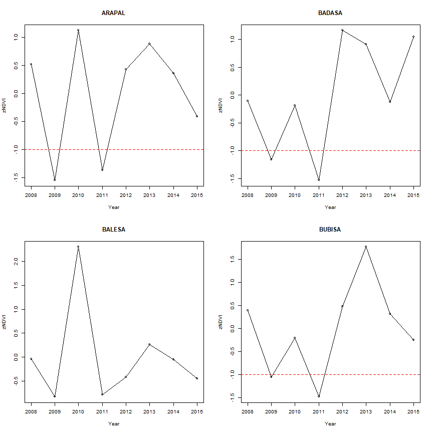
We can show z-scores over the analysis years per sub-region. Here for four regions
years <- 2008:2015
par(mfrow=c(2,2))
for(i in 1:4){
    plot(years, scores[i,], ylab="zNDVI", xlab="Year", main=pols$SUB_LOCATION[i])
    lines(years, scores[i,])
# Line showing where NDVi is 1 sd below the mean
    abline(h=-1, col="red",lty=2)
}