SI: Sustainable intensification
Adoption Pathways Project, Tanzania
In this case study, we will look at survey data and replicate summary statistics from the Adoption Pathways project in East Africa, part of a larger project on sustainable intensification research led by CIMMYT. This project consists of panel data from five countries in the region between 2010 and 2015. In this case study, we will look at data from Tanzania only, beginning with the 2010 survey.
2010 Data
The dataset, available on dataverse here, is organized into eleven parts with several sections in each. The dataset includes surveys and supplementary documents, totaling 38 individual files. In this section, we will replicate a few of the results from the 2010 Household Baseline Report, which can be found in the dataset. This report calculates basic summary statistics, which are displayed with various charts and graphs.
There are two surveys included in the dataset: a household level survey, and a community level survey. These surveys include the questionnaires that were given to individuals and households in the field. In order to make sense of the variables listed in each table, we need to refer to the questionnaire. Each part and section of the questionnaire corresponds to a different table in the dataset. In this example, we will be looking at the household level questionnaire.
Because we begin by observing and cleaning up the data, we want to read in all of the tables into our environment. The below code reads in multiple tables at once by using lapply and read.delim, and then names each of the files appropriately. We can then view each table by specifying the particular part and section of the survey where it originated from. For example, to see the first table, we specify the object (x) and the name of the table, such as “x$Part0”.
ff <- agro::get_data_from_uri("hdl:11529/10754", ".")
head(ff)
## [1] "./hdl_11529_10754/Community Baseline Report.doc"
## [2] "./hdl_11529_10754/Community_Level_Questionnaire_1.doc"
## [3] "./hdl_11529_10754/Data_Usage_Information_Form.txt"
## [4] "./hdl_11529_10754/Household Baseline Report.docx"
## [5] "./hdl_11529_10754/Household_Level_Questionnaire_1.docx"
## [6] "./hdl_11529_10754/Part 0 Interview background_1.tab"
length(ff)
## [1] 38
#Creates a list of files with the pattern .tab
ff <- grep('\\.tab$', ff, value=TRUE)
#Use lapply to read in each file from the above list
x <- lapply(ff, read.delim)
#The next section cleans up the names of each of the tables that were read in above.
z <- strsplit(basename(ff), ' ')
z <- t(sapply(z, function(x) x[1:4]))
z[z[,3]!='Section', 4] <- ""
z <- apply(z[,-3], 1, function(i) paste(i, collapse=""))
names(x) <- z
###Sample Location We will begin our analysis be summarizing the number of households in each district. The houeshold level questionannaire begins with an interview background which includes questions about the location of each household, including the zone, region, and district. We are able to find relevant variables by matching the survey questions with the variable names in Part 0. The districts are recorded as values from 1-4, and by comparing to the quantities listed in the report we can deduce which district is given which value. The results differ slightly from those reported in table 1 of the baseline report.
#create a factor of district
district <- as.factor(x$Part0$district2)
#Name each level according to the district name, for clarity.
levels(district) <- c("Karatu", "Mbulu", "Mvomero", "Kilosa")
summary(district)
##  Karatu   Mbulu Mvomero  Kilosa
##     164     185     135     217
###Household Demographic Characteristics Next, we replicate a few of the summary statistics from table 2 of the baseline report, which show household demographic characteristics.Because the questions are asked to all individuals within a household, we get a subset of the data that only contains information from the household heads. Then, we can calculate the average household size, sex of household head, education level, and age. Household size needs to be calcuulated, which we can do by counting the number of people with each household ID using the table function.
#To only get a subset of the data which is the information on household heads
 HH <- x$Part2[x$Part2$relnhhead=="1",]
#Add district information to the household head data
HH$district <- as.factor(x$Part0$district2)
levels(HH$district) <- c("Karatu", "Mbulu", "Mvomero", "Kilosa")
#Household Size:
count <- as.data.frame(table(x$Part2$hhldid))
#Add this as a new column to household heads
HH$size <- count$Freq
#Household Age: there is one age recorded as -77, we convert this to NA
HH$age[HH$age==-77] <- NA
#Use aggregate to find the mean of multiple columns (sex, age, education, and size) in the data frame by district
table <- aggregate(HH[,c(3,6, 19, 7)], list(HH$district), mean, na.rm=T)
table[,2:5] <- round(table[,2:5], 2)
#transpose so that it matches the table in the report
tablet <- t(table)
tabled <- as.data.frame(tablet[-1,])
# the first row will be the header
colnames(tabled) <- c("Karatu", "Mbulu", "Mvomero", "Kilosa")
tabled$Average  <- apply(na.omit(HH[,c(3,6, 19, 7)]), 2, mean)
tabled[,5] <- round(tabled[,5], 2)
rownames(tabled) <-c("Male headed household", "Age of Household Head (years)", "Household Size (number)", "Education of Household Head (years)")
library(knitr)
kable(tabled)
Karatu |
Mbulu |
Mvomero |
Kilosa |
Average |
|
|---|---|---|---|---|---|
Male headed household |
0.88 |
0.90 |
0.84 |
0.88 |
0.88 |
Age of Household Head (years) |
50.09 |
43.43 |
47.35 |
44.06 |
45.93 |
Household Size (number) |
6.00 |
6.22 |
4.95 |
5.07 |
5.57 |
Education of Household Head (years) |
5.09 |
5.34 |
5.65 |
5.20 |
5.31 |
###Main occupation of household head on average by district: Next, we want to find the main occupation of the household heads in each district. The variable “mainoccup” is a factor variable with numbers cooresponding to different occupations. From the questionnaire provided, we are able to identify what each factor in the variable titled “mainoccup” corresponds to (Codes E on page 3 of the survey), such as farming, salaried employment, or casual laborer. We then organize this information into a single dataframe, with the code below.
library(dplyr)
occupation <- as.factor(HH$mainoccup)
levels(occupation) = c("Other", "Farming(crop+livestock)", "Salaried Employment", "Self-employed off-farm", "Casual labourer off-farm", "Other", "Other")
 #this gives us a count
occupationtab <-  as.data.frame(table(occupation, district))
occupationtab <- reshape(occupationtab, timevar="district", idvar="occupation", direction= "wide")
occupationtab <- occupationtab[,-1]
#To cacluate percentages of each column, we can use the mutate function in the dplyr package.
occupationtab <- mutate(occupationtab,
                Karatu = Freq.Karatu / sum(Freq.Karatu),
                Mbulu = Freq.Mbulu / sum(Freq.Mbulu),
                Mvomero = Freq.Mvomero/sum(Freq.Mvomero),
                Kilosa = Freq.Kilosa/sum(Freq.Kilosa))
#Remove count values and round
occupationtab <- round(occupationtab[,5:8],2)
#name the rows
rownames(occupationtab) <-levels(occupation)
#To get number of individuals dedicated to each occupation from all households
occupationall <- table(occupation)
occupationall <- round((occupationall/710)*100, 1)
occupationtab$Average <- occupationall
#To change the order to match the chart
occupationtab <- occupationtab[c(2,3,4,5,1), ]
#To display the chart
kable(occupationtab)
Karatu |
Mbulu |
Mvomero |
Kilosa |
Average |
|
|---|---|---|---|---|---|
Farming(crop+livestock) |
0.89 |
0.91 |
0.97 |
0.96 |
92.3 |
Salaried Employment |
0.06 |
0.06 |
0.00 |
0.01 |
3.5 |
Self-employed off-farm |
0.04 |
0.02 |
0.02 |
0.01 |
2.1 |
Casual labourer off-farm |
0.01 |
0.01 |
0.00 |
0.00 |
0.3 |
Other |
0.01 |
0.00 |
0.01 |
0.01 |
0.6 |
###Access to Health Services Another summary statistic we can calculate is access to health services. Questions about health services were asked in Part 1 of the survey, Farmers Identification and Village Characteristics, so we locate the appropriate variabels in the table Part1.
#Extract all variables into single dataframe
health <- x$Part1[,c("dtshlthc", "wlkminhl", "dstmnsrc", "wlkminsrcdrwtr")]
health[health<0] <- NA
#add district information
health$district <- as.factor(x$Part0$district2 )
levels(health$district) <- c("Karatu", "Mbulu", "Mvomero", "Kilosa")
#Use aggregate to see on average the access to health services by district
healtht <- aggregate(health[,1:4], list(district), mean, na.rm=T)
healtht[,2:5] <- round(healtht[,2:5], 2)
healtht <- t(healtht)
colnames(healtht) <- healtht[1,]
healtht <- healtht[-1,]
healtht <- as.data.frame(healtht)
#Next, we get the health variables for all the observations together
totalh  <-as.data.frame(apply(na.omit(health[1:4]), 2, mean))
healtht$Average <- round(totalh[,1], 2)
rownames(healtht) <- c("Distance to health center", "Time to health center", "Distance to drinking water", "Time to drinking water")
#To view the dataframe
kable(healtht)
Karatu |
Mbulu |
Mvomero |
Kilosa |
Average |
|
|---|---|---|---|---|---|
Distance to health center |
4.77 |
6.17 |
4.78 |
5.04 |
5.22 |
Time to health center |
61.06 |
57.46 |
61.02 |
56.81 |
59.11 |
Distance to drinking water |
3.89 |
1.79 |
1.09 |
0.95 |
1.90 |
Time to drinking water |
21.29 |
22.01 |
14.37 |
15.77 |
18.43 |
2013 Data
The next survey data was collected in 2013, and can be downloaded here
library(agro)
ff <- get_data_from_uri("hdl:11529/10755", ".")
head(ff)
## [1] "./hdl_11529_10755/Adoption Pathways Project Survey Report_shad_geoff (Final_6March2015).docx"
## [2] "./hdl_11529_10755/Data_Usage_Information_Form.txt"
## [3] "./hdl_11529_10755/Module 10-Part A _  Role in household decision making.tab"
## [4] "./hdl_11529_10755/Module 10-Part B _  Role in household decision making _ Continued.tab"
## [5] "./hdl_11529_10755/Module 11 _ Leadership and influence in the community.tab"
## [6] "./hdl_11529_10755/Module 1 Household and village identification_1.tab"
length(ff)
## [1] 36
The 2013 questionnaire has a similar format to 2010, but many of the questions have been updated and adjusted. Additionally, there is some attrition, and the district of Kilosa has been split into two separate districts, Gairo and Kilosa. All of these issues make for more challenging analysis of trends across the years.
First, we read in the data with code similar to that used above for the 2010 data.
ff2 <- grep('\\.tab$', ff, value=TRUE)
x2 <- lapply(ff2, read.delim)
#To name each of the tables
z2 <- strsplit(basename(ff2), " |-")
z2 <- t(sapply(z2, function(x2) x2[1:4]))
z2[1,3] <- "Part"
z2[1, 4] <- "A"
z2[2,3] <- "Part"
z2[2,4] <- "B"
z2[z2[,3]!='Part', 4] <- ""
z2 <- apply(z2[,-3], 1, function(i) paste(i, collapse=""))
names(x2) <- z2
Attrition Rate
To find the attrition rate, we can summarize the number of observations per district each year, then use the cbind function to combine the results from each year.
#the fist section creates a matrix that tells us the number of people interviewed by district
district13 <- as.factor(x2$Module1B$district2)
levels(district13) <- c("Karatu", "Mbulu", "Mvomero", "Kilosa")
district13.count <- as.matrix(summary(district13), byrow=T)
#then I do the same for the 2010 data
district10 <- as.factor(x$Part0$district2)
levels(district10) <- c("Karatu", "Mbulu", "Mvomero", "Kilosa")
district10.count <- as.matrix(summary(district10), byrow=T)
#combine the two matrices into one table
attrition <- as.data.frame(cbind(district13.count, district10.count))
#add the column names
colnames(attrition) <- c("N_2010", "N_2013")
#formula to add column for attrition rate
attrition$percent_attrition <- (((attrition$N_2010-attrition$N_2013)/attrition$N_2010)*100)
#rounding
attrition$percent_attrition <- round(attrition$percent_attrition, 2)
knitr::kable(attrition)
N_2010 |
N_2013 |
percent_attrition |
|
|---|---|---|---|
Karatu |
0 |
164 |
-Inf |
Mbulu |
0 |
185 |
-Inf |
Mvomero |
0 |
135 |
-Inf |
Kilosa |
0 |
217 |
-Inf |
Household Demographic Information, 2013
To get information on households and household heads, we take a subset of only household heads from the original table. We create a new dataframe, HH2. Next, using similar code to the 2010 data, we can find basic demographic information from the households.
#same as 2010 data, I want to only see data on household heads
HH2 <- x2$Module2A[x2$Module2A$relnhhead == 1,]
#RH error here
HH2$district <- as.factor(x2$Module1B$district2)
levels(HH2$district) <- c("Karatu", "Mbulu", "Mvomero", "Kilosa")
count2 <- as.data.frame(table(x2$Module2A$hhldid))
#again, to get a count of number of people per household
HH2$size <- count2$Freq
table2 <- aggregate(HH2[,c(3, 6, 8, 32)], list(HH2$district), mean, na.rm=T)
table2[,2:5] <- round(table2[,2:5], 2)
tablet2 <- t(table2)
tabled2 <- as.data.frame(tablet2)
colnames(tabled2) <- c("Karatu", "Mbulu", "Mvomero", "Kilosa")  # the first row will be the header
tabled2 <- tabled2[-1, ]
tabled2
We can also calculate basic demographic information by gender of household head.
HH2$district <- x2$Module1B$district2
table3<-aggregate(HH2[,c(6, 8, 32)], list(HH2$sex), mean, na.rm=T)
table3[,2:4] <- round(table3[,2:4], 2)
tablet3 <- t(table3)
tabled3 <- as.data.frame(tablet3[-1,])
colnames(tabled3) <- c("Female", "Male")
tabled3
Food Security Measures
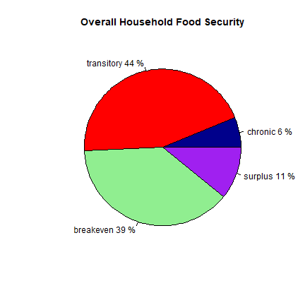
Next, we graph overall food security status, showing the percent of households in each designation of food security status.
#View(x2$Module9)
#To get one response per household
foodin <- x2$Module9[x2$Module9$qnntype == 1, c("chronic", "transitory", "breakeven", "surplus")]
#Use`apply` to count the number of individuals in each category
slices <- apply(foodin, 2, sum)
#we can use this information to create the pie chart
pct <- round(slices/sum(slices)*100)
#create labels
lbls <- paste(colnames(foodin), pct, "%", sep = " ")
color <- c("darkblue", "red", "lightgreen", "purple")
pie(slices, labels = lbls, col = color, main = "Overall Household Food Security")
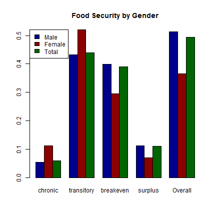
Using this food secuirty data, we can show the food security by gender in a barplot:
#extract information on food security from household heads
foodin2 <- x2$Module9[x2$Module9$qnntype == 1, c(21, 24, 25, 26, 27)]
gender <- as.factor(foodin2$sexhhead)
levels(gender) <- c("Female", "Male")
#food security by gender
tables <- aggregate(foodin2, list(gender), sum, na.rm=T)
foodsec<-as.matrix(tables[,3:6])
#The next code creates a new matrix that is the proportion of total for each cateogry of food security
Diagonal_Matrix <- diag(1/rowSums(foodsec))
#Then, we can multiply the proportion of each catogory by the number in each category to get percent food secure in each category
foodsec.pct <- Diagonal_Matrix %*% foodsec
#Here we add the total food security status, without gender
foodsec.pct <- rbind(foodsec.pct, pct/100)
#To change order of rows to match
foodsec.pct <- foodsec.pct[c(2,1,3),]
rownames(foodsec.pct) <- c("Male", "Female", "Total")
#To get total food security for male, female, and both
overall <- cbind(foodin2[,2]+foodin2[,3], foodin2[,4]+foodin2[,5])
colnames(overall) <- c("insecure", "secure")
overall <- data.frame(overall)
overall$gender <- gender
ag <- aggregate(overall[,1:2], list(gender), sum, na.rm=T)
ag$total <- ag$insecure + ag$secure
#first row is male secure, second is female secure, third is total secure
overall.list <-as.data.frame(c((ag[2,3]/ag[2,4]), (ag[1,3]/ag[1,4]), ((ag[1,3]+ag[2,3])/(ag[1,4]+ag[2,4])) ))
colnames(overall.list) <- "Overall"
foodsec.pct <- cbind(foodsec.pct, overall.list)
foodsec.pct <- as.matrix(foodsec.pct)
#Add the barplot
barplot(foodsec.pct, beside=T, main="Food Security by Gender", col=c("darkblue", "darkred", "darkgreen"))
legend("topleft", rownames(foodsec.pct), fill=c("darkblue", "darkred", "darkgreen"))
#And, to see the values:
kable(foodsec.pct)
chronic |
transitory |
breakeven |
surplus |
Overall |
|
|---|---|---|---|---|---|
Male |
0.0546218 |
0.4327731 |
0.3991597 |
0.1134454 |
0.5126050 |
Female |
0.1126761 |
0.5211268 |
0.2957746 |
0.0704225 |
0.3661972 |
Total |
0.0600000 |
0.4400000 |
0.3900000 |
0.1100000 |
0.4936015 |
2015 Data
Finally, we add the data from 2015.
library(agro)
ff <- get_data_from_uri("hdl:11529/11128", ".")
head(ff)
## [1] "./hdl_11529_11128/Module 10 PART A CREDIT NEED AND SOURCES.dta"
## [2] "./hdl_11529_11128/Module 10 Part B saving.dta"
## [3] "./hdl_11529_11128/Module 10 Part C ACCESS TO EXTENSION SERVICES.dta"
## [4] "./hdl_11529_11128/Module 10 Part D PRODUCTION EQUIPMENT AND MAJOR HOUSEHOLD FURNITURE..dta"
## [5] "./hdl_11529_11128/Module 11 PART A LIVESTOCK OWNERSHIP, MARKETING AND PRODUCTION.dta"
## [6] "./hdl_11529_11128/Module 12 HOUSEHOLD INCOME FOR THE LAST 12 MONTHS.dta"
length(ff)
## [1] 26
This data is primarily stored as .dta files, which are used in Stata. However, because four of the files are .tab, we read in the two file types separately, and append the lists together.
#For the .tab files:
ff3 <- grep('\\.tab$', ff, value=TRUE)
x3 <- lapply(ff3, read.delim)
z3 <- strsplit(basename(ff3), ' ')
z3 <- t(sapply(z3, function(x3) x3[1:4]))
z3[1,4] <- "A1"
z3[2,4] <- "A2"
z3[3,4] <- "A"
z3[z3[,3]!='Part', 4] <- ""
z3 <- apply(z3[,-3], 1, function(i) paste(i, collapse=""))
names(x3) <- z3
#For the .dta files:
library(foreign)
ff4 <- grep('\\.dta$', ff, value=TRUE)
x4 <- lapply(ff4, read.dta)
z4 <- strsplit(basename(ff4), ' ')
z4 <- t(sapply(z4, function(x4) x4[1:4]))
#This particular table had multiple parts combined, and is simplier without the commas.
z4[13,4] <- "BCD"
z4[z4[,3] != 'Part', 4] <- ""
z4 <- apply(z4[,-3], 1, function(i) paste(i, collapse=""))
names(x4) <- z4
#To combine the .tab and .dta files into a single object
x3 <- append(x3, x4)
It appears that the number of households in 2015 actually increased in two of the districts from 2013, shown by the negative attrition values in the chart below. However, there are fewer respondants than 2010, meaning that not all of the original respondants have been interviewed in the third phase of the panel data collection.
#There are 26 NA entries at the end of this table, so we wish to remove them.
HH3 <- x3$Module2A2[!is.na(x3$Module2A2$relnhhead ),]
HH3$realid <- HH3$hhldid
comb <- merge(HH3, HH, by="hhldid")
HH3$district <- comb$district
district15 <- as.factor(HH3$district)
district15.count <- as.matrix(summary(district15), byrow=T)
attrition <- as.data.frame(cbind(district13.count, district10.count, district15.count))
#add the column names
colnames(attrition) <- c("N_2010", "N_2013", "N_2015")
#formula to add column for attrition rate
attrition$attrition_since_2010 <- (((attrition$N_2010-attrition$N_2015)/attrition$N_2010)*100)
attrition$attrition_since_2013 <- (((attrition$N_2013-attrition$N_2015)/attrition$N_2010)*100)
#rounding
attrition$attrition_since_2010 <- round(attrition$attrition_since_2010, digits=2)
attrition$attrition_since_2013 <- round(attrition$attrition_since_2013, digits=2)
kable(attrition)
N_2010 |
N_2013 |
N_2015 |
attrition_since_2010 |
attrition_since_2013 |
|
|---|---|---|---|---|---|
Karatu |
0 |
164 |
151 |
-Inf |
Inf |
Mbulu |
0 |
185 |
149 |
-Inf |
Inf |
Mvomero |
0 |
135 |
101 |
-Inf |
Inf |
Kilosa |
0 |
217 |
182 |
-Inf |
Inf |
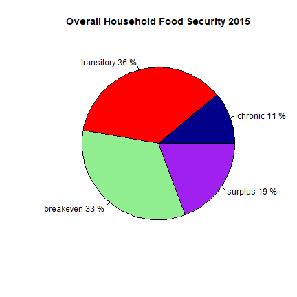
Food Security Pie Chart
Like we did with the 2010 data, we can create a pie chart that shows the portion that are food secure. However, the data for 2015 is organized differently than it was for 2010. The data from 2010 had a different column for each food security level (chronic, transitory, breakeven, surplus), and each column contained a value of 0 or 1 depeneding on if the household fit the level. The 2015 data has a single column that states the food security level of each household.
foodin15 <- x3$MODULE9[x3$MODULE9$Respondent_type=="Primary (main respondent)",]
slices15 <- summary(na.omit(foodin15$M9_PA_15))
lbls <- c("chronic", "transitory", "breakeven", "surplus")
pct15 <- round(slices15/sum(slices15)*100)
lbls <- paste(lbls, pct15, "%",sep=" ")
color <- c("darkblue", "red", "lightgreen", "purple")
pie(slices15, labels=lbls, col=color, main= "Overall Household Food Security 2015")
Analysis of panel data
Many of the same questions were asked in the surveys from each of the three years, although the format of the responses and the structure of the tables, including the names of variables, has changed significantly. Using this panel data, we can analyze how some of the household characteristics have changed over time. While we would expect basic demographics such as education and age to increase within the same households, we could also assess whether there have been increases in adoption of improved maize varities, or changes in the food security of households.
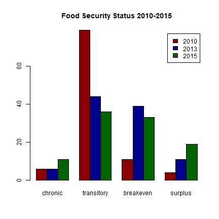
Food security over the years
Using the panel data, we can observe how food security status changes over the three years the survey was taken. It is interesting to note that each of the three datasets organizes the food security data in a slightly different way. 2010 data uses a numeric code, 2013 data has separate columns for each food security status, and 2015 data uses a character description. It appears from basic summary statistics that food insecurity is decreasing, but not for those who are chronically food insecure.
foodsec10 <- x$Part1$fmlfoodc
#The 2010 food security data is coded as numbers from 1-4. Numbers outside this range are errors and are NA.
foodsec10[foodsec10>4 | foodsec10<1] <- NA
k <- as.data.frame(table(foodsec10))
slices10 <- k$Freq
pct10 <- round(slices10/sum(slices10)*100)
pctcomb <- data.frame(pct10, pct, pct15)
pctcomb <- t(pctcomb)
colnames(pctcomb) <- c("chronic", "transitory", "breakeven", "surplus")
rownames(pctcomb) <- c("2010", "2013", "2015")
barplot(pctcomb, beside=T, legend.text=row.names(pctcomb), col=c('darkred', 'darkblue', 'darkgreen'), main="Food Security Status 2010-2015")
Fertilizer Use
Next, we can look at fertilizer use across the three years in Tanzania. Each survey asked the same questions about fertilizer use on the plots, and used the same variable names to organize the data. We can use this to see the portion of households that used fertilizer, and to see whether this changes over time.
#2010 fertilizer
fert10 <- x$Part6B[x$Part6B$cropgrwn1 == 1,c("hhldid", "subplot", "amtplant", "cstpltfert", "amttopdr", "csttopdr")]
fert10[fert10 < 0] <- NA
fert10$quanttotal10 <- fert10$amtplant + fert10$amttopdr
fert10$fert10 <- pmin(1, fert10$amtplant + fert10$amttopdr)
summary(fert10$fert10)
##    Min. 1st Qu.  Median    Mean 3rd Qu.    Max.    NA's
## 0.00000 0.00000 0.00000 0.04376 0.00000 1.00000      41
fert10hh <- aggregate(fert10$fert10, by= list(fert10$hhldid), sum)
colnames(fert10hh) <- c("hhldid", "fert10")
fert10hh$fert10[fert10hh$fert10 > 1] <- 1
#2013 fertilizer
fert13 <- x2$Module3A1[x2$Module3A1$cropgrwn1 == 1, c("hhldid", "plotcode", "amtplant", "cstpltfert", "amttopdr", "csttopdr", "methpayfert")]
fert13[fert13 < 0] <- NA
fert13$quanttotal13 <- fert13$amtplant + fert13$amttopdr
fert13$fert13 <- pmin(1, fert13$amtplant + fert13$amttopdr)
summary(fert13$fert13)
##    Min. 1st Qu.  Median    Mean 3rd Qu.    Max.
## 0.00000 0.00000 0.00000 0.05409 0.00000 1.00000
fert13hh <- aggregate(fert13$fert13, by= list(fert13$hhldid), sum)
colnames(fert13hh) <- c("hhldid", "fert13")
fert13hh$fert13[fert13hh$fert13 > 1] <- 1
fert15 <- x3$Module3A[x3$Module3A$cropgrwn1 == 1,c("hhldid", "plotcode", "amtplant", "cstpltfert", "amttopdr", "csttopdr", "methpayfert")]
fert15[fert15 < 0] <- NA
fert15$quanttotal15 <- fert15$amtplant + fert15$amttopdr
fert15$fert15 <- pmin(1, fert15$amtplant + fert15$amttopdr)
summary(fert15$fert15)
##    Min. 1st Qu.  Median    Mean 3rd Qu.    Max.    NA's
## 0.00000 0.00000 0.00000 0.04439 0.00000 1.00000       3
fert15hh <- aggregate(fert15$fert15, by= list(fert15$hhldid), sum)
colnames(fert15hh) <- c("hhldid", "fert15")
fert15hh$fert15[fert15hh$fert15 > 1] <- 1
Now we combine data from all 3 years into a single dataframe. We want to retain as many observations as possible, so we use “all.x = T” and “all.y = T”.
fertall <- merge(fert10hh, fert13hh, all.x = TRUE, all.y = TRUE)
fertall <- merge(fertall, fert15hh, all.x = TRUE, all.y = TRUE)
increase <- fertall$fert15 > fertall$fert10
summary(increase)
##    Mode   FALSE    TRUE    NA's
## logical     515      18     167
decrease <-  fertall$fert15 < fertall$fert10
summary(decrease)
##    Mode   FALSE    TRUE    NA's
## logical     522      11     167
#how many years did the household use fertilizer
fertall$sum <- as.factor(fertall$fert10 + fertall$fert13 + fertall$fert15)
#did the household use fertilizer in any of the three years?
fertall$any <- pmin(1, fertall$fert10 + fertall$fert13 + fertall$fert15)
#We can see that the highest portion of households used fertilizer in 2013
summary(fertall[,c(2:4)])
##      fert10            fert13            fert15
##  Min.   :0.00000   Min.   :0.00000   Min.   :0.00000
##  1st Qu.:0.00000   1st Qu.:0.00000   1st Qu.:0.00000
##  Median :0.00000   Median :0.00000   Median :0.00000
##  Mean   :0.04525   Mean   :0.06111   Mean   :0.05151
##  3rd Qu.:0.00000   3rd Qu.:0.00000   3rd Qu.:0.00000
##  Max.   :1.00000   Max.   :1.00000   Max.   :1.00000
##  NA's   :37        NA's   :160       NA's   :137