Maize Agronomy in Tanzania

Introduction

This case study looks looks at the data from the 2016 and 2017 Agronomy Panel Survey for Tanzania. This data is part of the household panel dataset under TAMASA, and includes agronomic, yield, and soil information. The dataset includes a farm and plot survey with sixteen sections, as well as a community level questionnaire. Additionally, an excel document is included that contains a description of the variable names.

In this case study we will calculate basic summary statistics and compare the two years of panel data. The data can be found on the CIMMYT webset, here and here.

Download the data

ff2016 <- agro::get_data_from_uri("hdl:11529/10548039", ".")
ff2017 <- agro::get_data_from_uri("11529/10548038", ".")
## Error in get_simple_URI(uri): Not valid unique object identifier (DOI or HDL)
ff2016
##  [1] "./hdl_11529_10548039/TZAPS16_cmty.tab"
##  [2] "./hdl_11529_10548039/TZAPS16_hhfp_fertavail.tab"
##  [3] "./hdl_11529_10548039/TZAPS16_hhfp_groupmemb.tab"
##  [4] "./hdl_11529_10548039/TZAPS16_hhfp_lstock.tab"
##  [5] "./hdl_11529_10548039/TZAPS16_hhfp_mroster.tab"
##  [6] "./hdl_11529_10548039/TZAPS16_hhfp_othinc.tab"
##  [7] "./hdl_11529_10548039/TZAPS16_hhfp_othinp.tab"
##  [8] "./hdl_11529_10548039/TZAPS16_hhfp_plotmcc.tab"
##  [9] "./hdl_11529_10548039/TZAPS16_hhfp_plotmc.tab"
## [10] "./hdl_11529_10548039/TZAPS16_hhfp_plotmlf.tab"
## [11] "./hdl_11529_10548039/TZAPS16_hhfp_plotmlh.tab"
## [12] "./hdl_11529_10548039/TZAPS16_hhfp_plotscc.tab"
## [13] "./hdl_11529_10548039/TZAPS16_hhfp_plotsc.tab"
## [14] "./hdl_11529_10548039/TZAPS16_hhfp_plotslf.tab"
## [15] "./hdl_11529_10548039/TZAPS16_hhfp_plotslh.tab"
## [16] "./hdl_11529_10548039/TZAPS16_hhfp_seed.tab"
## [17] "./hdl_11529_10548039/TZAPS16_hhfp.tab"
## [18] "./hdl_11529_10548039/TZAPS16_hhfp_weed.tab"
## [19] "./hdl_11529_10548039/TZAPS16_hh_plot.tab"
## [20] "./hdl_11529_10548039/TZAPS16_metadata.tab"
## [21] "./hdl_11529_10548039/TZAPS16_ODK_community.tab"
## [22] "./hdl_11529_10548039/TZAPS16_ODK_cs.tab"
## [23] "./hdl_11529_10548039/TZAPS16_ODK_hhpp.xls"
ff2017
## Error in eval(expr, envir, enclos): object 'ff2017' not found

Read in the data:

#2016 data
ff <- grep("\\.tab$", ff2016, value=TRUE)
x <- lapply(ff, read.delim)
z <- strsplit(basename(ff), '_|[.]')
z <- t(sapply(z, function(x) x[1:3]))
z[z[,3]=='tab', 3] <- ""
z <- apply(z[,-1], 1, function(i) paste(i, collapse="_"))
names(x)<-z
#2017 data
ff2 <- grep("\\.tab$", ff2017, value=TRUE)
## Error in eval(expr, envir, enclos): object 'ff2017' not found
x2 <- lapply(ff2, read.delim)
## Error in eval(expr, envir, enclos): object 'ff2' not found
z2 <- strsplit(basename(ff2), '_|[.]')
## Error in eval(expr, envir, enclos): object 'ff2' not found
z2 <- t(sapply(z2, function(x2) x2[1:3]))
## Error in eval(expr, envir, enclos): object 'z2' not found
z2[z2[,3]=='tab',3] <- ""
## Error: object 'z2' not found
z2 <- apply(z2[,-1], 1, function(i) paste(i, collapse=""))
## Error in eval(expr, envir, enclos): object 'z2' not found
names(x2) <- z2
## Error in eval(expr, envir, enclos): object 'z2' not found

We will need to use a few packages in this case study for mapping and graphics:

library(maptools)
## Loading required package: sp
## Checking rgeos availability: TRUE
## Please note that 'maptools' will be retired during 2023,
## plan transition at your earliest convenience;
## some functionality will be moved to 'sp'.
library(raster)
library(plyr)
library(ggplot2)
library(rgdal)
## Please note that rgdal will be retired during 2023,
## plan transition to sf/stars/terra functions using GDAL and PROJ
## at your earliest convenience.
## See https://r-spatial.org/r/2022/04/12/evolution.html and https://github.com/r-spatial/evolution
## rgdal: version: 1.6-6, (SVN revision 1201)
## Geospatial Data Abstraction Library extensions to R successfully loaded
## Loaded GDAL runtime: GDAL 3.6.2, released 2023/01/02
## Path to GDAL shared files: C:/soft/R/R-4.3.0/library/rgdal/gdal
##  GDAL does not use iconv for recoding strings.
## GDAL binary built with GEOS: TRUE
## Loaded PROJ runtime: Rel. 9.2.0, March 1st, 2023, [PJ_VERSION: 920]
## Path to PROJ shared files: C:/soft/R/R-4.3.0/library/rgdal/proj
## PROJ CDN enabled: FALSE
## Linking to sp version:1.6-0
## To mute warnings of possible GDAL/OSR exportToProj4() degradation,
## use options("rgdal_show_exportToProj4_warnings"="none") before loading sp or rgdal.

Because the dataset includes some lat/long data, we can plot the communities that were surveyed over a map of Tanzania. This way, we can see the geographical extent of the data.

latlong <- x$cmty_[, c("X_comm_gps_latitude","X_comm_gps_longitude")]
names(latlong) <- c("lat", "long")
latlong <- latlong [-2,]
#switch lat and long.. .they are in wrong place
latlong <- latlong[,c(2,1)]
points <- SpatialPoints(latlong)
latlong2 <- x2$cmty[,c("X_comm_gps_longitude", "X_comm_gps_latitude")]
## Error in eval(expr, envir, enclos): object 'x2' not found
names(latlong2) <- c("long", "lat")
## Error: object 'latlong2' not found
points2 <- SpatialPoints(latlong2)
## Error in h(simpleError(msg, call)): error in evaluating the argument 'obj' in selecting a method for function 'coordinates': object 'latlong2' not found
#get a map of tanzania, district level
Tanz<-getData("GADM", country="TZ", level=2)
## Warning in getData("GADM", country = "TZ", level = 2): getData will be removed in a future version of raster
## . Please use the geodata package instead
#plot the country with points to indicate where the communities are. Red indicates 2016 data, blue is 2017. The mostly overlap.
plot(Tanz)
points(points, col= "red")

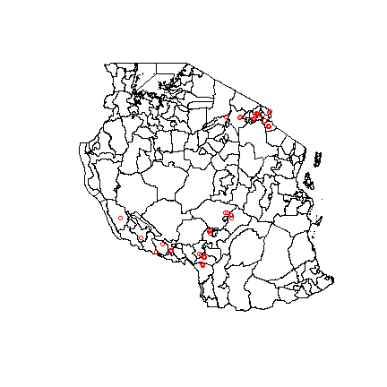
points(points2, col= "blue")
## Error in eval(expr, envir, enclos): object 'points2' not found

Next we can show basic plot characteristics.

plot <- x$hh_plot
plot <- plot[,c(2,6,7,8,13,20,22)]
colnames(plot) <- c("hhindex", "size", "unit", "distance", "ownership", "irrigation", "erosion_control")
plot$size <- ifelse(plot$unit == "hectare", plot$size*2.4, plot$size)
plot$unit <- NULL
plot$irrigation <- ifelse(plot$irrigation == "yes", 1, 0)
plot$erosion_control <- ifelse(plot$erosion_control == "yes", 1, 0)
colnames(plot) <- c("hhinex", "size(acres)", "distance(km)", "ownership", "irrigation (%)", "erosion (%)")
plotchars <- round(apply(plot[,c(2:3, 5:6)], 2, mean), 2)
kable(plotchars, caption= "Plot Characteristics")
## Error in kable(plotchars, caption = "Plot Characteristics"): could not find function "kable"
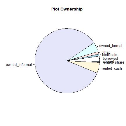
#Because the ownership information is qualitative, we can make a pie chart to represent the information:
c <- count(plot$ownership)
pie(c$freq, labels=c$x, main = "Plot Ownership")

The survey also includes information on basic household demographics, such as age of household head, education, sex, and marital status. Here we can demonstrate the basic information:

tamasa_hh <- x$hhfp_mroster
tamasa_hh2 <- x$hhfp_
tamasa_size <- tamasa_hh2[,c("hhid", "hh_index", "adults", "child10_15", "child10")]
tamasa_size$size <- tamasa_size$adults + tamasa_size$child10 + tamasa_size$child10_15
tamasa_size[,c(3:5)] <- NULL
colnames(tamasa_size) <- c("hhid", "hh_index", "size")
tamasa_HH2 <- tamasa_hh[tamasa_hh$mem_relationship=="head", c("hh_index", "mem_age", "mem_gender", "mem_education", "mem_marital")]
tamasa_HH <- merge(tamasa_size, tamasa_HH2, by="hh_index")
tamasa_HH$mem_gender <- ifelse(tamasa_HH$mem_gender=="female", 1, 0)
colnames(tamasa_HH) <- c("hh_index", "hhid", "size", "age", "sex", "education", "marital")
tamasa.mean <- apply(tamasa_HH[,3:5], 2, mean)
knitr::kable(tamasa.mean)

	x
size	5.7594502
age	48.4467354
sex	0.1271478

Fertilizer data:

tamasa_fert <- x$hhfp_
tamasa_fert <- tamasa_fert[,c("hhid", "fertilizer_bin", "why_not_fertilizer")]
tamasa_fert$fertilizer_bin <- ifelse(tamasa_fert$fertilizer_bin == "yes", 1, 0)
summary(tamasa_fert$fertilizer_bin)
##    Min. 1st Qu.  Median    Mean 3rd Qu.    Max.
##  0.0000  0.0000  0.0000  0.3987  1.0000  1.0000
#so here only 4 percent of households use fertilizer
summary(tamasa_fert$why_not_fertilizer)
##    Length     Class      Mode
##       607 character character
#we can add fertilizer information to the household data to see what variables may be correlated with fertilizer use
tamasa_all <- merge(tamasa_fert, tamasa_HH, by="hhid")
cor(tamasa_all$age, tamasa_all$fertilizer_bin)
## [1] -0.105008