Example run
Introduction
With WOFOST, crop growth is simulated using daily weather data parameters describing the crop(s) and soil type(s) of interest, as well as the crop management (such as planting date). You can calculate potential and water-limited production. In the current version, nutrient-limited production and yield reducing factors are not taken into account. In each model run, WOFOST simulates the growth of a specific crop, given the selected soil and weather data. For each simulation, you must select initial conditions such as the as the soil’s water status, and management decisions such as the crop planting date.
Chapter requirements
We use R package Rwofost. has been submitted to CRAN (March 2020),
so pretty soon you should be able install it
from there.
Input data
To run WOFOST, you need daily weather data. Here we
use an file that comes with the meteor package.
library(Rwofost)
## Warning: package 'Rwofost' was built under R version 4.3.1
f <- system.file("extdata/Netherlands_Swifterbant.csv", package="meteor")
wth <- read.csv(f)
wth$date <- as.Date(wth$date)
head(wth)
##         date srad tmin tmax  vapr wind prec
## 1 1974-01-01 1010 -4.3 -0.3 0.426  2.7    0
## 2 1974-01-02 2520 -3.8 -0.2 0.429  3.1    0
## 3 1974-01-03 2930 -0.2  2.7 0.536  4.0    0
## 4 1974-01-04 1030 -0.8  4.5 0.524  3.9    0
## 5 1974-01-05 2080  1.3  6.1 0.570  4.9    0
## 6 1974-01-06 2170  5.4  9.0 0.798  4.1    0
A variety is described by a (rather lengthy) set of crop
parameters. The Rwofost package comes with a set of
examples that you can use or build on. Let’s take barley
crop <- wofost_crop("barley")
We can also use example soil parameters.
soil <- wofost_soil('ec1')
And “control” parameters that set things like planting date.
contr <- wofost_control()
contr$modelstart <- as.Date("1976-02-06")
Model
Now that we have the input data we can either run the model in one step
out <- wofost(crop, wth, soil, contr)
Or in two steps, by first creating the model.
m <- wofost_model(crop, wth, soil, contr)
And then running it
d <- run(m)
A quick look at the output.
head(d)
## date step TSUM DVS LAI WRT WLV WST WSO TRA EVS
## 1 1976-02-06 1 0.00 0.0000000 0.048 36 24 0 0 0.0001000000 0.020965774
## 2 1976-02-07 2 0.00 0.0000000 0.048 36 24 0 0 0.0005782172 0.004506166
## 3 1976-02-08 3 0.00 0.0000000 0.048 36 24 0 0 0.0008030733 0.006081747
## 4 1976-02-09 4 1.45 0.0018125 0.048 36 24 0 0 0.0008149719 0.006953915
## 5 1976-02-10 5 3.80 0.0047500 0.048 36 24 0 0 0.0012147822 0.015495359
## 6 1976-02-11 6 7.65 0.0095625 0.048 36 24 0 0 0.0016005854 0.025690388
## EVW SM
## 1 0 0.11
## 2 0 0.11
## 3 0 0.11
## 4 0 0.11
## 5 0 0.11
## 6 0 0.11
tail(d)
## date step TSUM DVS LAI WRT WLV WST
## 156 1976-07-10 156 1452.05 1.860000 3.404459 923.0412 1289.4806 3117.727
## 157 1976-07-11 157 1468.80 1.882333 3.083766 904.5803 1173.4850 3057.122
## 158 1976-07-12 158 1485.40 1.904467 2.638628 886.4887 1014.7497 2997.304
## 159 1976-07-13 159 1504.95 1.930533 2.399597 868.7590 928.4277 2937.885
## 160 1976-07-14 160 1522.40 1.953800 2.174403 851.3838 846.2493 2879.131
## 161 1976-07-15 161 1539.40 1.976467 1.882020 834.3561 737.4964 2821.643
## WSO TRA EVS EVW SM
## 156 7700.983 0.2067904 0.02699927 0 0.11
## 157 7781.730 0.2972130 0.04686385 0 0.11
## 158 7854.682 0.3453991 0.07278994 0 0.11
## 159 7890.568 0.1046368 0.02183678 0 0.11
## 160 7890.914 0.1602666 0.04042056 0 0.11
## 161 7904.336 0.2197685 0.06898159 0 0.11
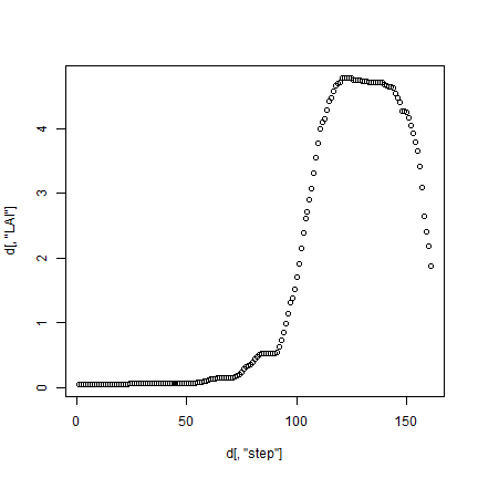
plot(d[,'step'], d[, 'LAI'])