The QUEFTS model
Introduction
This chapter describes the QUEFTS model. QUEFTS stands for
QUantitative Evaluation of the Fertility of Tropical Soils. It is a
rule-based model that can be used to estimate crop yield from soil
properties, the amount of fertilizer applied, and an estimate of the
yield that could be obtained when soil nutrients are in ample supply. It
can also be used to estimate the amount of fertilizer needed to reach a
particular yield. QUEFTS was first described by Janssen et al.,
1990.
See Sattari et al.,
2014
for an evaluation and updates of the model.
To run QUEFTS for a particular location, you need data on local soil quality, and we discuss these first. You also need crop parameters and the location specific attainable yield. In this context, attainable yield is the yield that would be reached if crop growth is not limited by low levels the three macro-nutrients nitrogen (N), phosphoros (P) and potassium (K).
Native soil supply of nutrients
The first step in using a QUEFTS model is to estimate the native soil supply of the three macro-nutrients N, P, K. Other nutrients are ignored here, although the model could be extended to include them.
The native supply of nutrients is the amount that is availble to a crop when no fertilizer is applied to the soil. The native nutrient supply is estimated from chemical properties of the topsoil.
The equations used by QUEFTS to calculate the native supply of nutrients from soil properties were derived from empirical data of field trials in Suriname and Kenya. They were thought to be applicable to well drained, deep soils, that have a pH(H20) in the range 4.5-7.0, and values for organic carbon below 70 g/kg, P-Olsen below 30 mg/kg and exchangeable potassium below 30 mmol/kg Janssen et al., 1990. Sattari et al., 2014 expanded the equations to be applicable to a wider range of conditions, and we will use these improved equations here.
Below we compute the nutrient supply for a location with an average temperature of 25C, a pH of 6, the organic C concentration is 10 g/kg, and exchangeable potassium is 1 mmol/kg. Phosphorus extracted with the Olsen method is 10 mg/kg; and the total amount of P is is 500 mg/kg.
library(Rquefts)
## Warning: package 'Rquefts' was built under R version 4.3.1
s <- nutSupply2(temp=25, pH=6, SOC=15, Kex=1, Polsen=10, Ptotal=500)
s
##      N_base_supply P_base_supply K_base_supply
## temp      76.03381            12      18.32258
We see that the soils supply of N is 76 kg/ha, that the P supply is 12 kg/ha, and the K supply is 18 kg/ha.
Now let’s compute nutrient supply across a range of pH values, keeping the other values constant.
ph <- seq(from=4.5, to=8.5, by=0.1)
s <- nutSupply2(temp=25, pH=ph, SOC=15, Kex=1, Polsen=10, Ptotal=500)
phs <- cbind(ph, s)
head(phs)
##       ph N_base_supply P_base_supply K_base_supply
## [1,] 4.5      41.14771          5.14      25.80645
## [2,] 4.6      41.14771          5.14      25.20894
## [3,] 4.7      41.14771          5.14      24.61142
## [4,] 4.8      43.83126          6.26      24.01390
## [5,] 4.9      46.51480          7.38      23.41639
## [6,] 5.0      49.19835          8.50      22.81887
par(mfrow=c(1,3))
plot(phs[, c(1,2)])
plot(phs[, c(1,3)])
plot(phs[, c(1,4)])
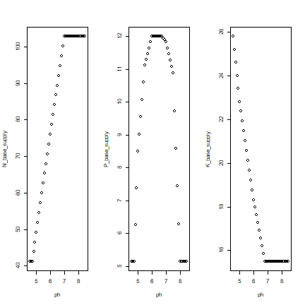
We see that the pH affters the supply of nutruents in different ways for N, P, and K. The P-supply is highest at a pH=6 – reflecting the fact that phosphoros becomes less available to plants at low or high pH. N-supply decreases with pH (everything else, such as the amount of soil carbon, being equal), and K-supply increases with pH (given the amount of exchangeble K).
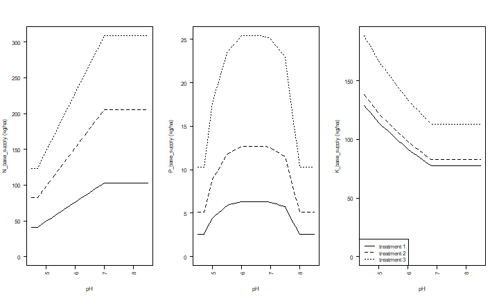
Let’s do this once, more but with different levels of some of the other properties.
s1 <- nutSupply2(25, ph, SOC=15, Kex=5,  Polsen=5, Ptotal=5*55)
s2 <- nutSupply2(25, ph, SOC=30, Kex=10, Polsen=10, Ptotal=10*55)
s3 <- nutSupply2(25, ph, SOC=45, Kex=20, Polsen=20, Ptotal=20*55)
We can use the results to make plots of the effect of pH on N, P and K supply, for these three situations (low, medium and high levels of organic matter, exchangeble K, and Olsen-P).
par(mfrow=c(1,3))
sup <- c("N_base_supply", "P_base_supply", "K_base_supply")
for (i in 1:3) {
  yb <- paste(sup[i],"(kg/ha)")
  ym <- c(0, max(s3[, sup[i]]))
  plot(ph, s1[,sup[i]], xlab="pH", ylab=yb, type="l", ylim=ym, lty=1, las=2)
  lines(ph, s2[, sup[i]], lty=2)
  lines(ph, s3[, sup[i]], lty=3)
}
legend("bottomleft", paste("treatment", 1:3), lty=1:3)
Now let’s look at the nutrient supply for differnt levels of soil Carbon.
# unit is g/kg
om <- seq(0, 70, 5)
# three combinations
s1 <- nutSupply2(temp=25, pH=5.5, SOC=om, Kex=5, Polsen=5, Ptotal=5*55)
s2 <- nutSupply2(temp=25, pH=5.5, SOC=om, Kex=10, Polsen=10, Ptotal=10*55)
s3 <- nutSupply2(temp=25, pH=5.5, SOC=om, Kex=20, Polsen=20, Ptotal=20*55)
# and plot
par(mfrow=c(1,3))
for (supply in c("N_base_supply", "P_base_supply", "K_base_supply")) {
  plot(om, s3[,supply], xlab="Soil Carbon (g/kg)", ylab=paste(supply, "(kg/ha)"), type="l", ylim=c(0,max(s3[,supply])), lty=1)
  lines(om, s2[,supply], lty=2)
  lines(om, s1[,supply], lty=3)
}
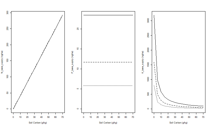
This shows that organic carbon has a strong positive effect on available N and P, but a negative effect on K availability (given the amount of exchangable K).
To use QUEFTS we need to assume that these relationships are robust — that is, not too far off. But with experimental data, these relationships could be re-estimated and improved.
Nutrient uptake and production
With the native soil nutrient supply, and possibly supply from fertilizer, QUEFTS computes the nutrient uptake by a crop, and from that it estimates crop yield.
Uptake of each nutrient is estimated from the soil supply of that nutrient, the supply of the other two nutrients, and the maximum nutrient concentrations in the vegetative and generative organs of the crop. These maximum concentrations are crop-specfic parameters that we will use below when we run the model.
The estimated uptake of N, P, and K is then used to estimated biomass production ranges for each nutrient. For each pair of nutrients two yield estimates are calculated. For example, production for the N uptake is dependent on the production range for the P and the for the K uptake. This leads to six combinations describing the uptake of one nutrient given maximum dilution or accumulation of another. The nutrient-limited production is then estimated by averaging these six estimates for paired nutrients. An estimate based on two nutrients may not exceed the upper limit of the yield range of the third nutrient, that is, the concentration of a nutrient cannot be lower than its maximum dilution level. Neither may the production estimates exceed the specified attainable (maximum) production.
Create and run a model
Quick start
To run QUEFTS, the first step is to create a model. You can create a model with default parameters like this
library(Rquefts)
q <- quefts()
And then run the model
run(q)
##   leaf_lim   stem_lim  store_lim   N_supply   P_supply   K_supply   N_uptake
## 1928.19667 1928.19667 3756.94929   90.00000   11.00000   90.00000   81.66872
##   P_uptake   K_uptake      N_gap      P_gap      K_gap
##   10.88951   77.38765   60.00000  205.00000    0.00000
Normally you would initialize a model with parameters of your choice.
Soil parameters
soil <- quefts_soil()
class(soil)
## [1] "list"
str(soil)
## List of 7
##  $ N_base_supply: num 60
##  $ P_base_supply: num 10
##  $ K_base_supply: num 60
##  $ N_recovery   : num 0.5
##  $ P_recovery   : num 0.1
##  $ K_recovery   : num 0.5
##  $ UptakeAdjust : num [1:7, 1:2] 0 40 80 120 240 360 1000 0 0.4 0.7 ...
soil$UptakeAdjust
##      [,1] [,2]
## [1,]    0  0.0
## [2,]   40  0.4
## [3,]   80  0.7
## [4,]  120  1.0
## [5,]  240  1.6
## [6,]  360  2.0
## [7,] 1000  2.0
We see that there are 7 soil parameters (one if which is a matrix). The first three give the native soil supply, as we discussed above. The “recovery” parameters set the fraction of avaiable nutrients that a crop may take up (the remainder is either lost or chemically or biologically captured). The UptakeAdjst matrix serves to adjust the nutrient availability given the length of the growing season. The standard season length is 120 days. The longer the season, the higher the total nutrient supply.
Crop parameters
The Rquefts package comes with a set of standard parameters for a number of crops. We get a list of them if we request a crop that does not exist.
quefts_crop(name="x")
## Error in quefts_crop(name = "x"): x not found. Choose from:
## Barley, Cassava, Chickpea, Chillies, Cotton, Cowpea, Field bean
## Groundnut, Jute, Kenaf, Lentil, Maize, Millet (bulrush), Mungbean
## Onion, Pigeonpea, Potato, Rapeseed, Rice, Sesame, Sorghum
## Soyabean, Sugarbeet, Sugarcane, Sunflower, Sweetpotato, Tobacco, Wheat
We’ll use barley
crop <- quefts_crop(name="Barley")
str(crop)
## List of 15
##  $ crop     : chr "Barley"
##  $ NminStore: num 0.011
##  $ NminVeg  : num 0.0035
##  $ NmaxStore: num 0.035
##  $ NmaxVeg  : num 0.012
##  $ PminStore: num 0.0016
##  $ PminVeg  : num 4e-04
##  $ PmaxStore: num 0.006
##  $ PmaxVeg  : num 0.0025
##  $ KminStore: num 0.003
##  $ KminVeg  : num 0.007
##  $ KmaxStore: num 0.008
##  $ KmaxVeg  : num 0.028
##  $ Yzero    : int 200
##  $ Nfix     : num 0
Again, we have a list of paramters. These are the mostly the minimum and maximum delution parameters, as described above, for the vegetative and generative (storage) organs, and for N, P, and K.
If the crop has biological nitrogen fixation (in symbiosis with Rhizobium) you can use the Nfix parameter to determine the fraction of the total nitrogen supply that is supplied by biological fixation. Note that Nfix is a constant, while in reality nitrogen fixation is amongst other things dependent on the amount of mineral nitrogen available in the soil.
Other parameters
You can set the fertilizer applied with a list like this
fertilizer <- list(N=50, P=0, K=0)
We set the attainable biomass accumlation to 2200 kg/ha for leaves, 2700 kg/ha for stems, and 4800 kg/ha for grain. All these numbers are expressed as dry matter weigts. As a rule of the thumb, for cereals, you can assume a harvest index of 0.5. That is, the grain yield is about half the biomass. The other half is divided by the leaves (45%) and stems (55%). We set the seasonlength to 110 days.
biomass <- list(leaf_att=2200, stem_att=2700, store_att=4800, SeasonLength=110)
Create model
And we can create a model with these parameters.
q <- quefts(soil, crop, fertilizer, biomass)
You can inspect the model with str (short for “structure”):
str(q)
## Reference class 'Rcpp_QueftsModel' [package "Rquefts"] with 9 fields
##  $ K           : num 0
##  $ N           : num 50
##  $ P           : num 0
##  $ SeasonLength: num 110
##  $ crop        :Reference class 'Rcpp_QueftsCrop' [package "Rquefts"] with 14 fields
##   ..$ KmaxStore: num 0.008
##   ..$ KmaxVeg  : num 0.028
##   ..$ KminStore: num 0.003
##   ..$ KminVeg  : num 0.007
##   ..$ Nfix     : num 0
##   ..$ NmaxStore: num 0.035
##   ..$ NmaxVeg  : num 0.012
##   ..$ NminStore: num 0.011
##   ..$ NminVeg  : num 0.0035
##   ..$ PmaxStore: num 0.006
##   ..$ PmaxVeg  : num 0.0025
##   ..$ PminStore: num 0.0016
##   ..$ PminVeg  : num 4e-04
##   ..$ Yzero    : num 200
##   ..and 16 methods, of which 2 are  possibly relevant:
##   ..  finalize, initialize
##  $ leaf_att    : num 2200
##  $ soil        :Reference class 'Rcpp_QueftsSoil' [package "Rquefts"] with 7 fields
##   ..$ K_base_supply: num 60
##   ..$ K_recovery   : num 0.5
##   ..$ N_base_supply: num 60
##   ..$ N_recovery   : num 0.5
##   ..$ P_base_supply: num 10
##   ..$ P_recovery   : num 0.1
##   ..$ UptakeAdjust : num [1:14] 0 40 80 120 240 360 1000 0 0.4 0.7 ...
##   ..and 16 methods, of which 2 are  possibly relevant:
##   ..  finalize, initialize
##  $ stem_att    : num 2700
##  $ store_att   : num 4800
##  and 18 methods, of which 4 are  possibly relevant:
##    finalize, initialize, run, runbatch
And you can inspect and change parameters.
q$N
## [1] 50
q$N <- 100
q$N
## [1] 100
model output
And, of course, you can run the model.
output <- run(q)
round(output, 1)
##  leaf_lim  stem_lim store_lim  N_supply  P_supply  K_supply  N_uptake  P_uptake
##    1354.8    1662.7    2877.4     105.5       9.2      55.5      95.6       9.0
##  K_uptake     N_gap     P_gap     K_gap
##      52.6      85.8     160.9     113.3
The results show the nutrient limited production of leaves, stems, and the storage organ, as well as the N, P, and K supply and uptake. The N, P, and K gap show the amounts of fertilizer that would be required to reach the attainable yield.
Explore
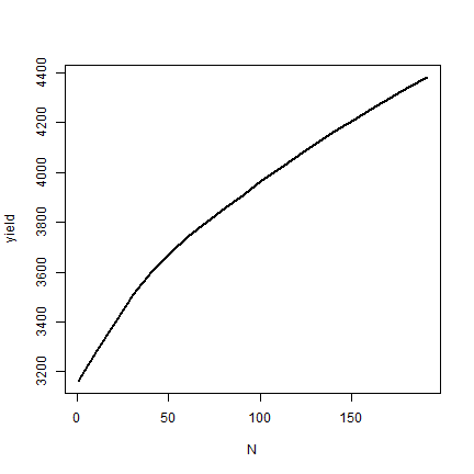
Let’s have a look how rice yield is affected by N fertilization. First set up some parameters
rice <- quefts_crop("Rice")
q <- quefts(crop=rice)
q$leaf_att <- 2651
q$stem_att <- 5053
q$store_att <- 8208
fert(q) <- list(N=0, P=0, K=0)
N <- seq(1, 200, 10)
Now set up an output matrix, and run the model for each fertlizer application.
results <- matrix(nrow=length(N), ncol=12)
colnames(results) <- names(run(q))
for (i in 1:length(N)) {
    q["N"] <- N[i]
    results[i,] <- run(q)
}
yield <- results[,"store_lim"]
yield
##  [1] 3162.406 3286.369 3402.153 3509.081 3604.427 3678.601 3744.550 3802.401
##  [9] 3858.675 3913.410 3966.648 4018.424 4068.778 4117.746 4165.363 4211.664
## [17] 4256.683 4300.454 4343.009 4384.379
And make a plot
plot(N, yield, type="l", lwd=2)
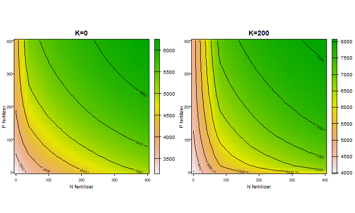
We can also look at interactions by changing two nutrients. Here we change N and P fertilization levels, while keeping K constant (either 0 or 200 mmol/kg)
f <- expand.grid(N=seq(0,400,10), P=seq(0,400,10), K=c(0,200))
x <- rep(NA, nrow(f))
for (i in 1:nrow(f)) {0
    q$N <- f$N[i]
    q$P <- f$P[i]
    q$K <- f$K[i]
    x[i] <- run(q)["store_lim"]
}
x <- cbind(f, x)
head(x)
##    N P K        x
## 1  0 0 0 3149.509
## 2 10 0 0 3274.362
## 3 20 0 0 3390.910
## 4 30 0 0 3498.943
## 5 40 0 0 3596.358
## 6 50 0 0 3671.320
To display the results we can treat the values as a raster
library(terra)
## terra 1.7.36
r0 <- rast(x[x$K==0, -3], type="xyz")
r200 <- rast(x[x$K==200, -3], type="xyz")
par(mfrow=c(1,2))
plot(r0, xlab="N fertilizer", ylab="P fertilizer", las=1, main="K=0")
contour(r0, add=TRUE)
plot(r200, xlab="N fertilizer", ylab="P fertilizer", las=1, main="K=200")
contour(r200, add=TRUE)
Callibration
If you have your own experimental data, you could callibrate QUEFTS. Here I illustrate some basic approaches that can be used for callibration.First I generate some data.
set.seed(99)
yldfun <- function(N, noise=TRUE) { 1000 +  500* log(N+1)/3 + noise * runif(length(N), -500, 500) }
N <- seq(0,300,25)
Y <- replicate(10, yldfun(N))
obs <- cbind(N, Y)
We will use Root Mean Square Error (RMSE) to assess model fit.
RMSE <- function(obs, pred) sqrt(mean((obs - pred)^2))
Let’s see how good the default parameters work for us.
q <- quefts()
q$P <- 0
q$K <- 0
results <- matrix(nrow=length(N), ncol=12)
colnames(results) <- names(run(q))
for (i in 1:length(N)) {
    q$N <- N[i]
    results[i,] <- run(q)
}
yield <- results[,'store_lim']
RMSE(obs[,-1], yield)
## [1] 1868.019
The RMSE is quite high.
We create a function to minimize with the optimizer. Here I try to improve the model by altering four parameters.
vars <- c('soil$N_base_supply', 'soil$N_recovery', 'crop$NminStore', 'crop$NmaxStore')
f <- function(p) {
    if (any (p < 0)) return(Inf)
    if (p['crop$NminStore'] >= p['crop$NmaxStore']) return(Inf)
    if (p['soil$N_recovery'] > .6 | p['soil$N_recovery'] < .3) return(Inf)
    q[names(p)] <- p
    pred <- run(q)
    RMSE(obs[,-1], pred['store_lim'])
}
# try the function with some initial values
x <- c(50, 0.5,  0.011, 0.035)
names(x) <- vars
f(x)
## [1] 1573.818
Now tht we have a working functon, we can use optimization methods to try to find the combination of parameter values that is the best fit to our data.
par <- optim(x, f)
# RMSE
par$value
## [1] 1478.384
# optimal parameters
par$par
## soil$N_base_supply    soil$N_recovery     crop$NminStore     crop$NmaxStore
##         0.01398939         0.59768399        26.37808069        37.05140516