QUEFTS

Introduction

This chapter describes the QUEFTS model. QUEFTS stands for QUantitative Evaluation of the Fertility of Tropical Soils. It is a simple rule-based model to estimate crop yield given the amount of fertilizer applied, or to estimate the amount of fertilizer needed to reach a particular yield.

To run the model, you need soil and crop parameters, as well as the amount of fertilizer applied, and the attainable crop biomass production. In this context, the attainable production that is either the maximum production in the absence of nutrient limitation, or another (lower) target biomass production.

QUEFTS was first described in: B.H. Janssen, F.C.T. Guiking, D. van der Eijk, E.M.A. Smaling, J. Wolf and H.van Reuler. 1990. A system for quantitative evaluation of the fertility of tropical soils (QUEFTS). Geoderma 46: 299-318.

Requirements

We will use the R package Rquefts. You can install it from CRAN.

if (!require(Rquefts)) { install.packages("Rquefts") }
library(Rquefts)

Technical background

Potential supply of nutrients

The model uses soil properties to estimate the potential soil supply of nitrogen (N), phosphorus (P) and potassium (K). This is done based on relationships between chemical properties of the topsoil and the maximum quantity of those nutrients that can be taken up by the crop, if no other nutrients limiting growth. This amount is crop and soil specific and can be determined through experiments where all other nutrients are in ample supply. The target nutrient thus becomes the most limiting, and the maximum soil supply of that nutrient can then be estimated from the crop’s nutrient uptake, and related to soil properties such as pH, and organic carbon content (Janssen et al., 1990). The equations used by QUEFTS to calculate the potential supplies of nutrients from soil properties were derived from empirical data of field trials in Suriname and Kenya. They are thought to be applicable to well drained, deep soils, that have a pH(H20) in the range 4.5-7.0, and values for organic carbon below 70 g/kg, P-Olsen below 30 mg/kg and exchangeable potassium below 30 mmol/kg.

Let’s have a look at this relationship. Below we compute the nutrient supply for a range of pH values, and given different levels for the other chemical properties.

library(Rquefts)
# range of pH values
ph <- seq(4, 8, 1)
s <- nutSupply(ph, SOC=1.5, Kex=1, Polsen=1)
cbind(ph, s)
##      ph N_base_supply P_base_supply K_base_supply
## [1,]  4          2.55       -0.0250     134.32836
## [2,]  5          5.10        0.7625     104.47761
## [3,]  6          7.65        1.0250      74.62687
## [4,]  7         10.20        0.7625      44.77612
## [5,]  8         12.75       -0.0250      14.92537

With a more detailed range of pH values, to make plots.

ph <- seq(4, 8, 0.25)
# three combinations
s1 <- nutSupply(ph, SOC=15, Kex=5, Polsen=5)
s2 <- nutSupply(ph, SOC=30, Kex=10, Polsen=10)
s3 <- nutSupply(ph, SOC=45, Kex=20, Polsen=20)

Now plots of the effect of pH on N, P and K supply, for three situations (low, medium and high levels of organic matter, exchangeble K, and Olsen-P).

par(mfrow=c(1,3))
for (supply in c("N_base_supply", "P_base_supply", "K_base_supply")) {
  plot(ph, s3[,supply], xlab="pH", ylab=paste(supply, "(kg/ha)"), type="l", ylim=c(0,max(s3[,supply])))
  lines(ph, s2[,supply])
  lines(ph, s1[,supply])
}

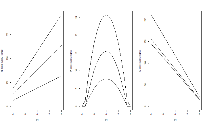
This shows that P-supply is highest at a pH=6, for any Olsen-P level. N-supply decreases with pH (given the amount of soil Carbon), and K-supply increases with pH (given the amount of exchangeble K).

Now let’s look at nutrient supply for varying levels of Soil Carbon.

# unit is g/kg
om <- seq(0, 70, 5)
# three combinations
s1 <- nutSupply(pH=5.5, SOC=om, Kex=5, Polsen=5)
s2 <- nutSupply(pH=5.5, SOC=om, Kex=10, Polsen=10)
s3 <- nutSupply(pH=5.5, SOC=om, Kex=20, Polsen=20)
# and plot
par(mfrow=c(1,3))
for (supply in c("N_base_supply", "P_base_supply", "K_base_supply")) {
  plot(om, s3[,supply], xlab="Soil Carbon (g/kg)", ylab=paste(supply, "(kg/ha)"), type="l", ylim=c(0,max(s3[,supply])))
  lines(om, s2[,supply])
  lines(om, s1[,supply])
}

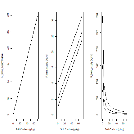
This shows that organic carbon has a strong positive effect on available N and P, but a negative effect on K availability (given the amount of exchangable K).

We can assume that these relationships are robust, at least for the conditions that they were designed for (pH(H20) 4.5-7.0, organic carbon below 70 g/kg, P-Olsen below 30 mg/kg and exchangeable potassium below 30 mmol/kg). But with more data, they could be re-estimated, also for other conditions.

Actual nutrient uptake

The actual uptake of each nutrient is estimated as a function of the potential soil supply of that nutrient, taking into account the potential soil supply of the other two nutrients, and the maximum nutrient concentrations in the vegetative and generative organs of the crop.

The estimated uptake of nitrogen, phosphorus, and potassium is used to estimated biomass production ranges for each nutrient. For each pair of nutrients two yield estimates are calculated. For example the yield for the actual N uptake is computed dependent on the yield range for the P uptake, and that for the actual P uptake in dependent on the yield range for the N uptake. This leads to six combinations describing the uptake of one nutrient given maximum dilution or accumulation of another.

The nutrient-limited yield is then estimated by averaging the six yield estimates for paired nutrients. An estimate based on two nutrients may not exceed the upper limit of the yield range of the third nutrient, that is, the concentration of a nutrient can not be lower than its maximum dilution level. Neither may the yield estimates exceed the spacified maximum (attainable) production.

TO DO: illustrate the procedure numerically and graphically

TO DO: discuss limitations based on the Sattari et al paper

Create and run a model

The first step is to create a model. You can create a model with default parameters like this

library(Rquefts)
q <- quefts()

And then run the model

run(q)
##   leaf_lim   stem_lim  store_lim   N_supply   P_supply   K_supply
## 1928.19667 1928.19667 3756.94929   90.00000   11.00000   90.00000
##   N_uptake   P_uptake   K_uptake      N_gap      P_gap      K_gap
##   81.66872   10.88951   77.38765   60.00000  205.00000    0.00000

You can also initialize a model with parameters of you choice

soiltype <- quefts_soil()
barley <- quefts_crop('Barley')
fertilizer <- list(N=50, P=0, K=0)
biomass <- list(leaf_att=2200, stem_att=2700, store_att=4800, SeasonLength=110)
q <- quefts(soiltype, barley, fertilizer, biomass)

TODO discuss parameters

If the crop has biological nitrogen fixation (in symbiosis with Rhizobium) you can use the NFIX parameter to determine the fraction of the total nitrogen supply that is supplied by biological fixation. Note that NFIX is a constant, while in reality nitrogen fixation is amongst other things dependent on the amount of mineral nitrogen available in the soil.

Explore

library(Rquefts)
rice <- quefts_crop("Rice")
q <- quefts(crop=rice)
q$leaf_att <- 2651
q$stem_att <- 5053
q$store_att <- 8208
fert(q) <- list(N=0, P=0, K=0)
N <- seq(1, 200, 10)
results <- matrix(nrow=length(N), ncol=12)
colnames(results) <- names(run(q))
for (i in 1:length(N)) {
    q["N"] <- N[i]
    results[i,] <- run(q)
}
yield <- results[,"store_lim"]
par(mfrow=c(1,2))
plot(N, yield, type="l", lwd=2)
Efficiency = yield / N
plot(N, Efficiency, type="l", lwd=2)

f <- expand.grid(N=seq(0,400,10), P=seq(0,400,10), K=c(0,200))
x <- rep(NA, nrow(f))
for (i in 1:nrow(f)) {0
    q$N <- f$N[i]
    q$P <- f$P[i]
    q$K <- f$K[i]
    x[i] <- run(q)["store_lim"]
}
x <- cbind(f, x)
# display results
library(raster  )
r0 <- rasterFromXYZ(x[x$K==0, -3])
r200 <- rasterFromXYZ(x[x$K==200, -3])
par(mfrow=c(1,2))
plot(r0, xlab="N fertilizer", ylab="P fertilizer", las=1, main="K=0")
contour(r0, add=TRUE)
plot(r200, xlab="N fertilizer", ylab="P fertilizer", las=1, main="K=200")
contour(r200, add=TRUE)

#plot(stack(r0, r200))

Callibration

Here I illustrate some basic approaches that can be used for callibration. First I generate some data.

set.seed(99)
yldfun <- function(N, noise=TRUE) { 1000 +  500* log(N+1)/3 + noise * runif(length(N), -500, 500) }
N <- seq(0,300,25)
Y <- replicate(10, yldfun(N))
obs <- cbind(N, Y)

We will use Root Mean Square Error (RMSE) to assess model fit.

RMSE <- function(obs, pred) sqrt(mean((obs - pred)^2))

Let’s see how good the default parameters work for us.

q <- quefts()
q$P <- 0
q$K <- 0
results <- matrix(nrow=length(N), ncol=12)
colnames(results) <- names(run(q))
for (i in 1:length(N)) {
    q$N <- N[i]
    results[i,] <- run(q)
}
yield <- results[,'store_lim']
RMSE(obs[,-1], yield)
## [1] 1868.019

The RMSE is quite high.

Create a function to minimize with the optimizer. Here I try to improve the model by altering four parameters.

vars <- c('soil$N_base_supply', 'soil$N_recovery', 'crop$NminStore', 'crop$NmaxStore')
f <- function(p) {
    if (any (p < 0)) return(Inf)
    if (p['crop$NminStore'] >= p['crop$NmaxStore']) return(Inf)
    if (p['soil$N_recovery'] > .6 | p['soil$N_recovery'] < .3) return(Inf)
    q[names(p)] <- p
    pred <- run(q)
    RMSE(obs[,-1], pred['store_lim'])
}
# try the function with some initial values
x <- c(50, 0.5,  0.011, 0.035)
names(x) <- vars
f(x)
## [1] 1573.818

Now optimize

par <- optim(x, f)
# RMSE
par$value
## [1] 1478.384
# optimal parameters
par$par
## soil$N_base_supply    soil$N_recovery     crop$NminStore
##         0.01398939         0.59768399        26.37808069
##     crop$NmaxStore
##        37.05140516