Random Forest¶

RandomForest is one of the most widely used “machine-learning” regression methods. This chapters shows how to use the method and how to inspect and evaluate RandomForest models.

Chapter requirements¶

For this chapter you need the following R packages: randomForest, rpart, reagro, and agro. See these instructions for installing R packages.

library(agrodata)
library(agro)
library(randomForest)
library(rpart)

Data¶

To illustrate the use of Random Forest, we use some data from West Africa on soil fertility and crop response to fertilizer. These data are part of a larger study described in a forthcoming paper (Bonilla et al.).

d <- reagro_data("soilfert")
dim(d)
## [1] 1684   12
head(d)
##      temp precip ExchP TotK ExchAl TotN sand clay  SOC  pH AWC fert
## 1463   27   1260   933  120    610 1157   65   17 13.5 6.3  26  120
## 1464   27   1260   933  120    610 1157   65   17 13.5 6.3  26  120
## 1465   27   1260   933  120    610 1157   65   17 13.5 6.3  26  120
## 1466   27   1260   933  120    610 1157   65   17 13.5 6.3  26  120
## 1467   27   1260   933  120    610 1157   65   17 13.5 6.3  26  120
## 1468   27   1260   933  120    610 1157   65   17 13.5 6.3  26  120

We create two sub-datasets.

set.seed(2019)
i <- sample(nrow(d), 0.5*nrow(d))
d1 <- d[i,]
d2 <- d[-i,]

These are the variables we have.

variable	description
temp	Average temperature
precip	Annual precipitation
ExchP	Soil exchangeble P
TotK	Soil total K
ExchAl	Soil exchangeble Al
TotN	Soil total N
sand	Soil franction sand (%)
clay	Soil fraction clay (%)
SOC	Soil organic carbon (g/kg)
pH	Soil pH
AWC	Soil water holding capacity
fert	fertilizer (index) kg/ha

Classification and Regression Trees¶

Before we look at the RandomForest, we first consider what the forest is made up of: trees. Specifically, the Classification and Regression Trees (CART) algorithm.

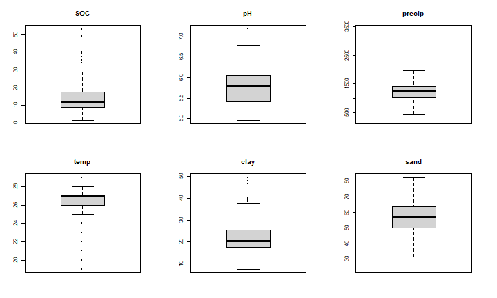
Suppose we were interested in estimating soil organic carbon (SOC) across locations in West Africa. Suppose we have a lot of data on soil pH and the fraction of the soil that is sand or clay (cheap and easy to measure), and precipitation and temperature data as well (which is available for any location). Can we build a model that predicts SOC from pH, sand and precipitation?

par(mfrow=c(2,3), mai=rep(0.5, 4))
for (v in c("SOC", "pH", "precip", "temp", "clay", "sand")) {
    boxplot(d[,v], main=v)
}

Let’s first make a linear regression model.

model <- SOC~pH+precip+temp+sand+clay
lrm <- lm(model, data=d1)
summary(lrm)
##
## Call:
## lm(formula = model, data = d1)
##
## Residuals:
##      Min       1Q   Median       3Q      Max
## -14.3389  -2.7321  -0.8637   1.8808  27.3512
##
## Coefficients:
##               Estimate Std. Error t value Pr(>|t|)
## (Intercept) -3.1972000  5.9665973  -0.536    0.592
## pH          -2.1496742  0.5405762  -3.977 7.59e-05 ***
## precip       0.0051574  0.0005337   9.663  < 2e-16 ***
## temp        -0.1058504  0.1675816  -0.632    0.528
## sand         0.1651263  0.0353392   4.673 3.46e-06 ***
## clay         0.7454555  0.0498190  14.963  < 2e-16 ***
## ---
## Signif. codes:  0 '***' 0.001 '**' 0.01 '*' 0.05 '.' 0.1 ' ' 1
##
## Residual standard error: 4.861 on 836 degrees of freedom
## Multiple R-squared:  0.5159, Adjusted R-squared:  0.513
## F-statistic: 178.2 on 5 and 836 DF,  p-value: < 2.2e-16
agro::RMSE_null(d2$SOC, predict(lrm, d2))
## [1] 0.3347983

We see that all the predictor variables are highly significant, and the R² is not that bad. Perhaps we could improve the model by including interaction terms, but let’s not go down that path here.

Instead we use CART. CART recursively partitions the data set using a threshold for one variable at a time to create groups that are as homogeneous as possible.

cart <- rpart::rpart(model, data=d1)
agro::RMSE_null(d2$SOC, predict(cart, d2))
## [1] 0.5883739

We see that RMSE_null is much better than the simple (perhaps overlay simplistic) linear model. CART explains about 58% of the unexplained variation, whereas the linear model explains only 21%. That is interesting. Let’s look at the model. We can inspect it like this.

plot(cart)
text(cart)

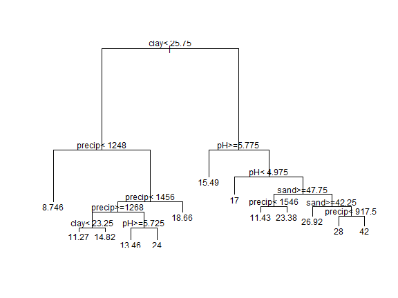
It may take a little effort at first, but once you get used to it, CART models are easy to understand. You can navigate down the tree. If the condition is true you go left, else you go right. So if clay < 25.75 and precip < 1248, SOC is predicted to be 8.7 (the value of the “leaf”. That is rather low (0.9% organic C, or about 1.5% soil organic matter) as might be expected on very sandy soil under relatively dry conditions. Notice how variables are used many times, in effect creating step-functions and interactions. Also note that with this tree, we end up with 13 possible predictions (the tree has 13 leaves).

We get a bit more detail, at the expense of visual pleasure, when we print the model like this.

cart
## n= 842
##
## node), split, n, deviance, yval
##       * denotes terminal node
##
##   1) root 842 4.081059e+04 13.906180
##     2) clay< 25.75 651 1.552559e+04 11.780340
##       4) precip< 1248 342 2.239368e+03  8.745614 *
##       5) precip>=1248 309 6.650516e+03 15.139160
##        10) precip< 1455.5 230 4.636887e+03 13.930430
##          20) precip>=1267.5 176 1.108358e+03 12.278410
##            40) clay< 23.25 126 5.853254e+02 11.269840 *
##            41) clay>=23.25 50 7.188000e+01 14.820000 *
##          21) precip< 1267.5 54 1.482648e+03 19.314810
##            42) pH>=5.725 24 9.583333e-01 13.458330 *
##            43) pH< 5.725 30 0.000000e+00 24.000000 *
##        11) precip>=1455.5 79 6.992722e+02 18.658230 *
##     3) clay>=25.75 191 1.231560e+04 21.151830
##       6) pH>=5.775 69 1.189746e+03 15.492750 *
##       7) pH< 5.775 122 7.666344e+03 24.352460
##        14) pH< 4.975 31 0.000000e+00 17.000000 *
##        15) pH>=4.975 91 5.419643e+03 26.857140
##          30) sand>=47.75 23 1.139435e+03 19.739130
##            60) precip< 1546.5 7 2.972143e+02 11.428570 *
##            61) precip>=1546.5 16 1.472500e+02 23.375000 *
##          31) sand< 47.75 68 2.720735e+03 29.264710
##            62) sand>=42.25 37 1.517568e+02 26.918920 *
##            63) sand< 42.25 31 2.122371e+03 32.064520
##             126) precip< 917.5 22 0.000000e+00 28.000000 *
##             127) precip>=917.5 9 8.705000e+02 42.000000 *

This shows, for example, that if we only used the first split (clay< 25.75), we get two groups. One group with 651 observations and a predicted (i.e., average) SOC of 11.8. The other group has 191 observations, and a predicted SOC of 21.2.

The big numbers express the remaining deviance (a goodness-of-fit statistic for a model). The Null deviance is 40810.6, but after the first split is has gone down to (15525 + 12315) = 27840.

The Null deviance can be computed like this

nulldev <- function(x) {
    sum((x - mean(x))^2)
}
nulldev(d1$SOC)
## [1] 40810.59

We can compare that with the deviance of the cart model.

cdev <- sum(cart$frame[cart$frame$var == "<leaf>", "dev"])
cdev
## [1] 6253.272
rdev <- round(100 * cdev / nulldev(d1$SOC))
rdev
## [1] 15

The model has reduced the deviance to 15%.

Let’s turn the data sets, and build a CART model with sub-dataset d2 (and evaluate with d1).

cart2 <- rpart::rpart(model, data=d2)
agro::RMSE_null(d1$SOC, predict(cart2, d1))
## [1] 0.5615755

That is very similar to the result for d1 (0.59). We can also check if the CART model overfits the data much by comparing RMSE computed with the test data with the RMSE computed with the train data.

# model 1, test data
agro::RMSE_null(d2$SOC, predict(cart, d2))
## [1] 0.5883739
# model 1, train data
agro::RMSE_null(d1$SOC, predict(cart, d1))
## [1] 0.6085582
# model 2, test data
agro::RMSE_null(d1$SOC, predict(cart2, d1))
## [1] 0.5615755
# model 2, train data
agro::RMSE_null(d2$SOC, predict(cart2, d2))
## [1] 0.6161892

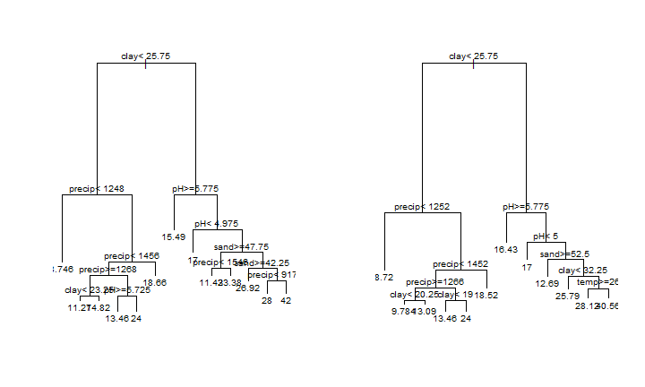
The rmse with the training data is higher than with the testing data. That suggest that there is some overfitting, but it is not much. In this case we also seem to have low variance, in the sense that the models look similar (see below). That is not a general result — CART models tend to have high variance. They can also overfit the data. A lot depends on how far you let the tree grow. In this case we used default stopping rules (nodes are not split if it has fewer than 20 observations or if any of the resulting nodes would get less than 7 observations), see ?rpart.control, that avoided these problems. Trees that are grown very deep tend to overfit: they have low bias, but very high variance.

par(mfrow=c(1,2))
plot(cart)
text(cart, cex=0.8)
plot(cart2)
text(cart2, cex=0.8)

CART models can be relatively easily inspected, and can “learn” about complex interactions. Another great feature is that they are not affected by the scale or transformation of the predictor variables. But they are prone to overfitting and instability. They are seldom accurate (Hastie et al.).

Random Forest¶

What is a Random Forest?¶

Random Forest builds many (> 100) CART models (we will call them trees) to create a new model that tends to have low variance, predict well, but does not overfit the data.

It would not be of any use to build the same tree 100s of times. Each tree is build with a bootstrapped sample of the records. A bootstrap sample is a random sample with replacement. Thus the number of records is the same for each tree, but some records are not included, and some records are included more than once. On average, about 2/3 of the records are included in a sample. Here is the computational proof of that:

mean(replicate(10000, length(unique(sample(100, replace=TRUE)))))
## [1] 63.3903

When a Random Forest model makes a prediction, a prediction is made for each tree, and the results are aggregated (averaged). This procedure of bootstrapping and aggregate, is called “bootstrap-aggregation” or “bagging”.

Let’s illustrate bagging by making 10 models with boostrapped data. Each model is used to make a prediction to test data, and evaluated.

n <- 10
set.seed(99)
predictions <- matrix(nrow=nrow(d2), ncol=n)
eval <- rep(NA, n)
for (i in 1:n) {
    k <- sample(nrow(d1), replace=TRUE)
    cartmod <- rpart(model, data=d1[k,])
    p <- predict(cartmod, d2)
    eval[i] <- agro::RMSE_null(d2$SOC, p)
    predictions[, i] <- p
}

For each “unseen” case in d2 we now have five predictions

head(predictions)
##          [,1]     [,2]     [,3]     [,4]     [,5]     [,6]     [,7]  [,8] [,9]
## [1,] 14.21875 13.89474 12.08462 14.68293 13.39655 11.04132 13.36364 13.54 13.5
## [2,] 14.21875 13.89474 12.08462 14.68293 13.39655 11.04132 13.36364 13.54 13.5
## [3,] 14.21875 13.89474 12.08462 14.68293 13.39655 11.04132 13.36364 13.54 13.5
## [4,] 14.21875 13.89474 12.08462 14.68293 13.39655 11.04132 13.36364 13.54 13.5
## [5,] 14.21875 13.89474 12.08462 14.68293 13.39655 11.04132 13.36364 13.54 13.5
## [6,] 14.21875 13.89474 12.08462 14.68293 13.39655 11.04132 13.36364 13.54 13.5
##         [,10]
## [1,] 12.18699
## [2,] 12.18699
## [3,] 12.18699
## [4,] 12.18699
## [5,] 12.18699
## [6,] 12.18699

We can average the individual model predictions to get our ensemble prediction.

pavg <- apply(predictions, 1, mean)

The quality of the individual models

round(eval, 3)
##  [1] 0.517 0.601 0.561 0.559 0.558 0.507 0.576 0.535 0.579 0.493

But the score for the ensemble model is quite a bit higher than the mean value is for the individual models!

mean(eval)
## [1] 0.5485663
agro::RMSE_null(d2$SOC, pavg)
## [1] 0.627291

And also higher than the original model (without bootstrapping)….

agro::RMSE_null(d2$SOC, predict(cart, d2))
## [1] 0.5883739

In Rob Shapire’s famous words: “many weak learners can make a strong learner”. (It would be nice if this is were not only true for statistical models, but that it would also hold for humans).

Random Forest has another randomization procedure. In a regression tree, the data is partitioned at each node using the best variable, that is, the variable that can most reduce the variance in the data. In Random Forest, only a random subset of all variables (for example one third) is available at each split (node). Although this further weakens the trees, it also makes them less correlated, which is a good feature (there is not much to gain from having many very similar trees).

Enough said. Let’s create a Random Forest model.

library(randomForest)
rf <- randomForest(model, data=d1)
rf
##
## Call:
##  randomForest(formula = model, data = d1)
##                Type of random forest: regression
##                      Number of trees: 500
## No. of variables tried at each split: 1
##
##           Mean of squared residuals: 5.165625
##                     % Var explained: 89.34

That’s it. Given reasonable software for data analysis, creating a machine learning model is just as complicated as creating a linear regression model. In this type of work the effort is to compile the data, to select a method, and to evaluate the results.

Compare reported results with ours

p <- predict(rf, d2)
agro::RMSE_null(d2$SOC, p)
## [1] 0.748259

# Mean of squared residuals
agro::RMSE(d2$SOC, p)^2
## [1] 3.051948
# % Var explained:
round(100 * (1 - var(d2$SOC - p) / var(d2$SOC)), 1)
## [1] 93.7

Cross validation¶

Instead of the data splitting that we used above, you always want to use the full dataset to fit your final model. The model that you will use. To evaluate the model, you should cross-validation.

In cross-validation the data is divided into k groups. Typically into 5 or 10 groups. Each group is used once for model testing, and k-1 times for model training. An extreme case that is “leave-one out”, where k is equal to the number of records, bu this is generally not considered a good practise.

Let’s make 5 groups.

n <- 5
set.seed(31415)
k <- agro::make_groups(d, n)
table(k)
## k
##   1   2   3   4   5
## 337 337 336 337 337

Now do the cross-validation, and compute a number of statistics of interest.

rfRMSE <- rfRMSE_null <- rfvarexp <- rfcor <- rep(NA, n)
for (i in 1:n) {
    test <- d[k==i, ]
    train <- d[k!=i, ]
    m <- randomForest(model, data=train)
    p <- predict(m, test)
    rfRMSE[i] <- agro::RMSE(test$SOC, p)
    rfRMSE_null[i] <- agro::RMSE_null(test$SOC, p)
    rfvarexp[i] <- var(test$SOC - p) / var(test$SOC)
    rfcor[i] <- cor(test$SOC, p)
}
mean(rfRMSE)
## [1] 1.602881
mean(rfRMSE_null)
## [1] 0.7708932
mean(rfvarexp)
## [1] 0.05427953
mean(rfcor)
## [1] 0.9741868

We can use the same procedure for any other predictive model. Here we show that for our linear regression model.

lmRMSE <- lmRMSE_null <- lmvarexp <- lmcor <- rep(NA, n)
for (i in 1:n) {
    test <- d[k==i, ]
    train <- d[k!=i, ]
    m <- lm(model, data=train)
    p <- predict(m, test)
    lmRMSE[i] <- agro::RMSE(test$SOC, p)
    lmRMSE_null[i] <- agro::RMSE_null(test$SOC, p)
    lmvarexp[i] <- var(test$SOC - p) / var(test$SOC)
    lmcor[i] <- cor(test$SOC, p)
}
mean(lmRMSE)
## [1] 4.738746
mean(lmRMSE_null)
## [1] 0.3169437
mean(lmvarexp)
## [1] 0.4654455
mean(lmcor)
## [1] 0.7329332

An important purpose of cross-validation is to get a sense of the quality of the model. But this is often not straighforward. Whether the quality of a model is sufficient depends on the purpose, and may require further numerical analysis.

Using cross-validation results is more straighforward in the context of model comparison. It can be used to select the best model, or, often more appropriate, to average a set of good models — perhaps a average weighted by the RMSE.

Cross-valdiation is important to find optimal values for “nuisance parameters” that needt to be set to regularize or otherwise parametrize a model. Examples for the randomForest methods are parameters such as ntry and nodesize. See ?randomForest.

Opening the box¶

Machine learning type regression models are sometimes described as “black boxes” — we cannot see what is going on inside. Afer all, we do not have a few simple parameters as we might have with a linear regression model. Well, the box has a lid, and we can look inside.

Here we show two general methods, “variable importance” and “partial response” that are available in for the R randomForest type models, but are really applicable to any predictive model.

Variable importance¶

Which variables are important, which are not?

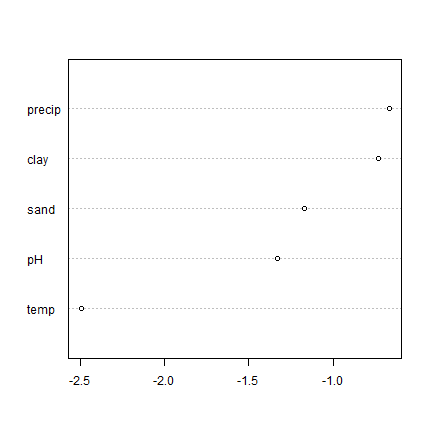
rfm <- randomForest(model, data=d)
varImpPlot(rfm)

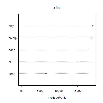
Intuitively this is very easy to understand: “clay” and “precip” are very important; “temp” is not. The “Increase in Node Purity” (IncNodePurity) expresses the change in the homogeneity of the of the groups created by the trees (using the Gini coefficient as a measure). What is expressed is the decrease in said purity if a particular variable has no information. If a variable has no information to begin with, the decrase would be zero.

The notion of node purity is specific to tree-models. But the notion of variable importance is not. We can also use the change in RMSE to look at variable importance.

Here is a general function that computes variable importance for any model (that has a “predict” methods) in R.

agro::varImportance
## function (mod, dat, vars, n = 10)
## {
##     rmse <- matrix(nrow = n, ncol = length(vars))
##     colnames(rmse) <- vars
##     for (i in 1:length(vars)) {
##         rd <- dat
##         v <- vars[i]
##         for (j in 1:n) {
##             rd[[v]] <- sample(rd[[v]])
##             p <- stats::predict(mod, rd)
##             rmse[j, i] <- RMSE(rd$SOC, p)
##         }
##     }
##     return(rmse)
## }
## <bytecode: 0x0000020283c16758>
## <environment: namespace:agro>

To assess importance for a variable, the function randomizes the values of that variable, without touching the other variables. It then use the model to make a prediction and compute a model evaluation statistic (here RMSE is used). Because of the vagaries of randomization this is done a number of times. The average RMSE is then compared with the RMSE of predictions with the original data. If the difference is large, the variable is important. If the difference is small, the variable is not important.

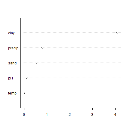
Now let’s use the function for our Random Forest model.

predvars <- c("pH", "precip", "clay", "sand", "temp")
vi <- agro::varImportance(rfm, d, predvars)
vimean <- colMeans(vi)
p <- predict(m, d)
RMSEfull <- agro::RMSE(d$SOC, p)
x <- sort(vimean - RMSEfull)
dotchart(x)

Not exactly the same as what varImpPlot gave us; but pretty much the same message.

We can use the same function for the linear regression model

mlr <- lm(model, data=d)
vi <- agro::varImportance(mlr, d, predvars)
vimean <- colMeans(vi)
p <- predict(m, d)
RMSEfull <- agro::RMSE(d$SOC, p)
x <- sort(vimean - RMSEfull)
dotchart(x)

Partial response plots¶

Another interesting concept is the partial response plot. It shows the response of the model to one variable, with the other variables held constant. (Although ALE plots may be a superior approach)

par(mfrow=c(2,2), mai=c(.75,rep(0.5,3)))
partialPlot(rfm, d, "pH")
partialPlot(rfm, d, "clay")
partialPlot(rfm, d, "sand")
partialPlot(rfm, d, "precip")

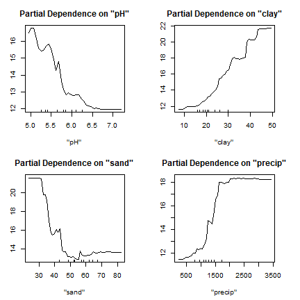
Do you think these responses make sense? That is, do they conform to what you know about soil science (if anything)?

You have to interpret these plots with caution as it does not show interactions; and these can be very important.

The partialPlot function comes with the randomForest package. Here is a generic implementation that works with any model with a predict method.

agro::partialResponse
## function (model, data, variable, rng = NULL, nsteps = 25)
## {
##     if (is.factor(data[[variable]])) {
##         steps <- levels(data[[variable]])
##     }
##     else {
##         if (is.null(rng)) {
##             rng <- range(data[[variable]])
##         }
##         increment <- (rng[2] - rng[1])/(nsteps - 2)
##         steps <- seq(rng[1] - increment, rng[2] + increment,
##             increment)
##     }
##     res <- rep(NA, length(steps))
##     for (i in 1:length(steps)) {
##         data[[variable]] <- steps[i]
##         p <- stats::predict(model, data)
##         res[i] <- mean(p)
##     }
##     data.frame(variable = steps, p = res)
## }
## <bytecode: 0x00000202835cd5a0>
## <environment: namespace:agro>

The function first creates a sequence of values for the variable of interest. It then loops over that sequence. In each iteration, all values for the variable of interest are replaced with a single value while the values of all other variables stay the same. The model is used to make a prediction for all records, and these predictions are averaged.

Let’s use it for pH with the Random Forest model

pr_pH <- agro::partialResponse(rfm, d, "pH")
plot(pr_pH, type="l")
rug(quantile(d$pH, seq(0, 1, 0.1)))

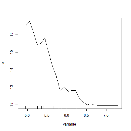
Very similar to what the partialPlot function returned.

And now for the linear regression model.

lrm <- lm(model, data=d)
pr_pH <- agro::partialResponse(lrm, d, "pH")
plot(pr_pH, type="l")
rug(quantile(d$pH, seq(0, 1, 0.1)))

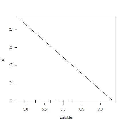
OK, that one is not too surprising. But it is nice that it works for any regression type model.

To do: show interactions

Conclusions¶

statistical modeling for inference is not the same as prediction
a major concern in prediction is the bias-variance trade-off (underfitting, overfitting)
predictive models are evaluated with cross-validation
cross-validation is also used to estimate (“nuisance”) parameters
there are general tools to inspect the properties of predictive models (variable importance, partial responses).
machine learning is easy to do, but harder to understand, at first
machine learning algorithms are not that hard to understand!

What we did not discuss¶

Random Forest can also do supervised classification (that is, predict classes) — see an example here.
Other examples:
Random Forest can also do unsupervised classification…

Citation¶

Hijmans, R.J., 2019. Statistical modeling. In: Hijmans, R.J. and J. Chamberlin. Regional Agronomy: a pratical handbook. CIMMYT. https:/reagro.org/tools/statistical/