Area yield insurance
Introduction
Here we consider an “area-yield” insurance contract that triggers if the average rice yield of an insurance zone is 10% below the zone’s long-term rice yield.
If yields are below this threshold, the contract makes payouts equivalent to the value of 90% of the zone’s long-term average yield minus the observed zonal rice yield for that season. The actual amount paid to a household depends on the area insured by a household.
Basics
First a refresher. Below y is a zone’s crop yield in season (time) t; and y_z is the zone’s long-term average rice yield. Yields are expressed in kg/ha.
get_payout <- function(y, y_z, trigger, price){
   pmax( (trigger * y_z) - y,  0) * price
}
To see how that works. Assume we observed the following sequence of rice yields.
yields <- seq(500, 2500, 100)
mean_yield <- mean(yields)
yields
##  [1]  500  600  700  800  900 1000 1100 1200 1300 1400 1500 1600 1700 1800 1900
## [16] 2000 2100 2200 2300 2400 2500
mean_yield
## [1] 1500
We set the rice price to $0.23 per kg.
price <- 0.23
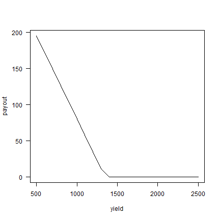
Now we can compute payouts
payout <- get_payout(yields, mean_yield, trigger=0.9, price=price)
plot(yields, payout, type="l", xlab="yield", ylab="payout", las=1)
If insurance did not cost any money, income could be computed like this.
rice_income <- yields * price
total_income <- rice_income + payout
plot(yields, total_income, type="l", xlab="yield", ylab="income", las=1)
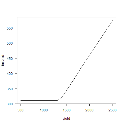
This shows that, thanks to insurance, income has a floor of $310.
The certainty equivalent without this insurance (not considering the premium, or other sources of income) would be
library(agrodata)
agro::ce_income(rice_income, rho=1.5)
## [1] 295.8926
And with insurance it would be
agro::ce_income(total_income, rho=1.5)
## [1] 375.0724
A more realistic situation might be a household that has additional income of $100 per year and that the insurance costs $50 per year.
rice_income <- yields * price
insurance_income <- payout - 50
total_income <- rice_income + insurance_income
agro::ce_income(rice_income, rho=1.5)
## [1] 295.8926
agro::ce_income(total_income, rho=1.5)
## [1] 323.1536
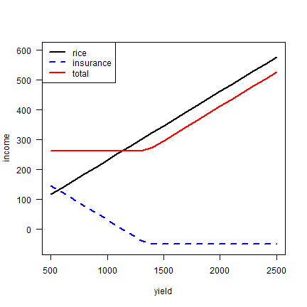
The certainly-equivalent income with insurance is still higher. We can plot that:
plot(yields, rice_income, type="l", xlab="yield", ylab="income", las=1, ylim=c(-60,600), lwd=2)
lines(yields, insurance_income, col="blue", lty=2, lwd=2)
lines(yields, total_income, col="red", lwd=2)
legend("topleft", c("rice", "insurance", "total"), col=c("black", "blue", "red"), lty=c(1,2,1), lwd=2)
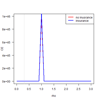
CE depends on rho
rho <- seq(0,3,.1)
ce_rice <- sapply(rho, function(r) agro::ce_income(rice_income, rho=r))
ce_tot <- sapply(rho, function(r) agro::ce_income(total_income, rho=r))
plot(rho, ce_rice, col="red", type="l", las=1, ylab="CE", lwd=2)
lines(rho, ce_tot, col="blue", lwd=2)
legend("topright", c("no inusrance", "insurance"), col=c("red", "blue"), lty=1, lwd=2 )
# certainty equivalents are the same at
i <- which.min(abs(ce_tot - ce_rice))
rho[i]
## [1] 0.3
abline(v=rho[i], lty=3, col="gray")
Tanzania households
Now get the household data from the previous chapter.
z <- readRDS("hh_rice_yield.rds")
head(z)
##      zone year        region fid        y  n y_zt  y_z y_dz
## 1 Maore N 2003 Northern_zone 208 3000.000 13 1360 1600 0.85
## 2 Maore N 2003 Northern_zone 228 1360.000 13 1360 1600 0.85
## 3 Maore N 2003 Northern_zone 267 2560.000 13 1360 1600 0.85
## 4 Maore N 2003 Northern_zone 275 1050.000 13 1360 1600 0.85
## 5 Maore N 2003 Northern_zone 255  840.000 13 1360 1600 0.85
## 6 Maore N 2003 Northern_zone 215 1923.077 13 1360 1600 0.85
Compute payouts per ha for each zone.
z$payout <- get_payout(z$y_zt, z$y_z, 0.9, price)
head(z)
##      zone year        region fid        y  n y_zt  y_z y_dz payout
## 1 Maore N 2003 Northern_zone 208 3000.000 13 1360 1600 0.85   18.4
## 2 Maore N 2003 Northern_zone 228 1360.000 13 1360 1600 0.85   18.4
## 3 Maore N 2003 Northern_zone 267 2560.000 13 1360 1600 0.85   18.4
## 4 Maore N 2003 Northern_zone 275 1050.000 13 1360 1600 0.85   18.4
## 5 Maore N 2003 Northern_zone 255  840.000 13 1360 1600 0.85   18.4
## 6 Maore N 2003 Northern_zone 215 1923.077 13 1360 1600 0.85   18.4
Now we can compute an insurance premium (per ha) for each zone z. First we determine the actuarially fair price where the premiums paid are equal to the expected value of compensation (payouts) paid.
pay_ha_year <- tapply(z$payout, z$year, mean)
pay_ha_year
##      2003      2004      2005      2006      2007      2008      2009      2010
## 14.083087  0.427141  2.942412  6.951119 46.973121  0.000000  2.379310  0.000000
##      2011      2012
##  0.000000 17.541482
afp <- mean(pay_ha_year)
afp
## [1] 9.129767
Let’s assume a markup of 20% (per ha)
premium <- round(afp, 1) * 1.2
premium
## [1] 10.92
income
For each household we can now compute income with and without insurance.
z$income <- z$y * price
z$income_with_ins <- z$income + z$payout - premium
head(z)
##      zone year        region fid        y  n y_zt  y_z y_dz payout   income
## 1 Maore N 2003 Northern_zone 208 3000.000 13 1360 1600 0.85   18.4 690.0000
## 2 Maore N 2003 Northern_zone 228 1360.000 13 1360 1600 0.85   18.4 312.8000
## 3 Maore N 2003 Northern_zone 267 2560.000 13 1360 1600 0.85   18.4 588.8000
## 4 Maore N 2003 Northern_zone 275 1050.000 13 1360 1600 0.85   18.4 241.5000
## 5 Maore N 2003 Northern_zone 255  840.000 13 1360 1600 0.85   18.4 193.2000
## 6 Maore N 2003 Northern_zone 215 1923.077 13 1360 1600 0.85   18.4 442.3077
##   income_with_ins
## 1        697.4800
## 2        320.2800
## 3        596.2800
## 4        248.9800
## 5        200.6800
## 6        449.7877
certainty equivalents by household
hh <- aggregate(z[, c("income", "income_with_ins")], z[,"fid", drop=FALSE], function(i) agro::ce_income(i, 1.5))
hh$benefit <- (hh$income_with_ins - hh$income)
hh$rel_benefit <- hh$benefit/ hh$income
head(hh)
##   fid   income income_with_ins    benefit  rel_benefit
## 1   4 131.7353        225.3080  93.572694  0.710308520
## 2   5 512.1919        500.4867 -11.705170 -0.022853097
## 3   6 828.1967        817.1718 -11.024975 -0.013312024
## 4   7 883.3441        885.5298   2.185758  0.002474413
## 5   8 274.1715        263.1199 -11.051632 -0.040309187
## 6   9 187.1586        175.7295 -11.429099 -0.061066393
mean(hh$benefit)
## [1] 6.934037
quantile(hh$benefit)
##         0%        25%        50%        75%       100%
## -66.480544 -10.356437  -4.081677   4.582311 340.715845
So, at the individual level, the contract meets the welfare test if you use the mean, but not if you use the median.
certainty equivalents by zone
zz <- aggregate(z[, c("income", "income_with_ins")], z[,"zone", drop=FALSE], function(i) agro::ce_income(i, 1.5))
zz$benefit <- (zz$income_with_ins - zz$income)
zz$rel_benefit <- zz$benefit/ zz$income
head(zz)
##       zone   income income_with_ins    benefit  rel_benefit
## 1  Maore N 157.2417        219.4529  62.211188  0.395640493
## 2 Maore SE 261.7988        255.2649  -6.533827 -0.024957441
## 3 Maore SW 193.5088        213.3387  19.829944  0.102475686
## 4 Ndungu E 253.1700        250.9713  -2.198716 -0.008684741
## 5 Ndungu N 301.5164        305.4767   3.960330  0.013134708
## 6 Ndungu S 214.4688        191.5201 -22.948608 -0.107002102
mean(zz$benefit)
## [1] 17.48121
quantile(zz$benefit)
##         0%        25%        50%        75%       100%
## -22.948608  -5.414573  10.599094  45.428325  62.211188
barplot(sort(zz$rel_benefit), ylab="relative benefit", xlab="zone", las=1)
So, at the zone level, the contract meets the welfare test both for the mean and the median (at rho=1.5).