Certainty equivalence
Introduction
Certainty equivalence is a key concept in evaluating insurance programs. It expresses the value of an uncertain stream of income (one year you earn more, another year you earn less) in terms of a stable income (you get the same income every year). For most people, a stable income is preferable to an unstable income, even if that unstable income is (somewhat) higher on average. This is because of the having a year with a low income can have a great negative effect on your welfare. In the extreme case you may die in a bad year for not being able to buy food.
How much lower the value of a variable income is relative to a stable income depends on your ability to protect yourself from the risk of a bad year. You may have a savings account, or family that can help you out. Another way to cope with risk is insurance. Certainty equivalence can be computed with a utility function.
Utility
The relationship between income and utility can be expressed with a utility function. In essence, a utility function expresses the diminishing returns to increased income. That is, if your income goes from $100 to $300 that could change your life, you gain a lot more additional utility than if goes from $4000 to $4300. How much exactly is hard to say. It depends on your preferences and circumstances.
For an insurance perspective, it is more useful to think about gaining versus loosing an amount of money. Imagine you have an income of $1000 per month. And where you live that is enough to pay for rent, food, and other basic needs; but for nothing more, you cannot save any money. If for some reason your boss would give you another $500 that would be great. You could spend it on something you like, perhaps some nice clothes, or to eat out, or to travel to see a family member. But now imagine that the company you work for is not doing well, and your boss takes away $500 of your monthly salary. That could be dramatically bad. You may be able to pay for food for your children; or for rent, and you may need to move in with relatives. In this case, the utility of $500 is asymetric, you get much more pain from loosing $500 than pleasure from gaining that amount of money. This dread of loosing relatively to gaining a certain amount of money implies that you are risk-adverse.
Utility functions are mathematical contructs that helps us reason about risk and estimate benefits of strategies to diminish it. Below is a common formulation of a utility function.
where U is the utility derived from income y, and \(\rho\) (rho) expresses the degree to which is loss of income is differnecece from a gain in income. In the context of insurance, this expresses the degree of risk aversion. If rho is zero, there is no difference between an amount lost or gained. The larger rho is the larger that difference.
Below you can see how this is expressed as a R function in the agrins package. Note that we add an option to scale the values between zero and one — to make it easier to plot them.
library(agro)
utility
## function (income, rho, scale = FALSE)
## {
##     income <- pmax(1, income)
##     rho[rho == 1] <- 0.99
##     u <- (income^(1 - rho))/(1 - rho)
##     if (scale) {
##         u <- u - min(u)
##         u <- u/max(u)
##     }
##     u
## }
## <bytecode: 0x000001b964991178>
## <environment: namespace:agro>
Let’s make a plot to illustrate the effect of changing \(\rho\).
income <- seq(1,1000,10)
rhos <- c(0, 0.5, 1, 1.5)
cols <- rainbow(4)
plot(NA, xlim=range(income), ylim=c(0,1), xlab="income", ylab="utility", type="n", las=1)
for (i in 1:length(rhos)) {
    u <- utility(income, rhos[i], scale=TRUE)
    lines(income, u, col=cols[i], lwd=2)
}
legend("bottomright", legend=rhos, col=cols, lty=1, lwd=2, title="rho")
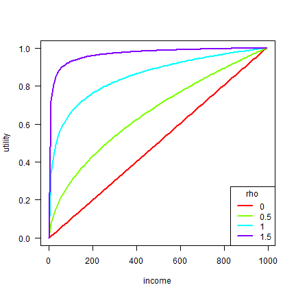
Higher values of rho correspond to higher levels risk aversion. But the utility values themselves have no direct meaning. They are used as weights in assessing the effect of income changes on welfare.
Let’s put this in perspective with some income data for households A and B. The have the same mean income over 10 years. The income for household A varies, that for household B is always the same.
A <- seq(100, 1000, 100)
B <- rep(mean(A), 5)
A
##  [1]  100  200  300  400  500  600  700  800  900 1000
B
## [1] 550 550 550 550 550
We can now compute the utilities of these income stream. Here we use
rho=1.5
uA <- utility(A, rho=1.5)
uB <- utility(B, rho=1.5)
round(mean(uA), 3)
## [1] -0.1
round(mean(uB), 3)
## [1] -0.085
The average utility for household B is higher than for household A.
Utilties are odd things to compare as they have no direct absolute interpretation. It is more useful to express them as certainty equivalents instead.
Certainty equivalent
A certainty equivalent expresses the value of a variable income in the equivalent income if it were stable. It can be computed from utility like this
agro::ce_utility
## function (utility, rho)
## {
##     u <- mean(utility)
##     if (rho == 1) {
##         exp(u)
##     }
##     else {
##         ((1 - rho) * u)^(1/(1 - rho))
##     }
## }
## <bytecode: 0x000001b9671598f8>
## <environment: namespace:agro>
But we will use the agro::ce_income function instead to compute
certainty equivalents directly from income.
agro::ce_income
## function (income, rho)
## {
##     u <- utility(income, rho, scale = FALSE)
##     ce_utility(u, rho)
## }
## <bytecode: 0x000001b964f07790>
## <environment: namespace:agro>
Back to households A and B. Let’s compute their certainty equivalent incomes.
ceA <- agro::ce_income(A, rho=1.5)
ceB <- agro::ce_income(B, rho=1.5)
ceA
## [1] 396.6614
ceB
## [1] 550
The certainty equivalent for B is $550 (because their income is always 550, 550, 550, 550, 550), but for household A it is $396.661382.
Let’s see how this depends on rho.
library(agro)
rho <- seq(0, 5, .1)
cerho <- sapply(rho, function(i) ce_income(A, i))
plot(rho, cerho, las=1, ylab="CE", type="l")
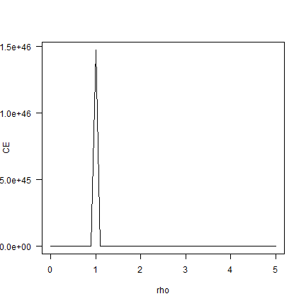
If you have no risk-aversion (rho=0) the certainty equivalent is the
same as the mean income. As rho increases, the CE approaches the
minimum income. Note that the shape of this curve is influenced by the
variation in income. The less variation, the flatter the curve.